suppressPackageStartupMessages({
library(recipes)
library(tidyverse)
library(embed)
library(ggforce)
library(tidymodels)
library(mixOmics)
library(fastICA)
library(bestNormalize)
})
theme_set(cowplot::theme_cowplot())
options(repr.plot.width=15,repr.plot.height=9)

Dimensionality Reduction

Dataset

library(beans)

head(beans)

A tibble: 6 × 17

area	perimeter	major_axis_length	minor_axis_length	aspect_ratio	eccentricity	convex_area	equiv_diameter	extent	solidity	roundness	compactness	shape_factor_1	shape_factor_2	shape_factor_3	shape_factor_4	class
<dbl>	<dbl>	<dbl>	<dbl>	<dbl>	<dbl>	<dbl>	<dbl>	<dbl>	<dbl>	<dbl>	<dbl>	<dbl>	<dbl>	<dbl>	<dbl>	<fct>
28395	610.291	208.1781	173.8887	1.197191	0.5498122	28715	190.1411	0.7639225	0.9888560	0.9580271	0.9133578	0.007331506	0.003147289	0.8342224	0.9987239	seker
28734	638.018	200.5248	182.7344	1.097356	0.4117853	29172	191.2728	0.7839681	0.9849856	0.8870336	0.9538608	0.006978659	0.003563624	0.9098505	0.9984303	seker
29380	624.110	212.8261	175.9311	1.209713	0.5627273	29690	193.4109	0.7781132	0.9895588	0.9478495	0.9087742	0.007243912	0.003047733	0.8258706	0.9990661	seker
30008	645.884	210.5580	182.5165	1.153638	0.4986160	30724	195.4671	0.7826813	0.9766957	0.9039364	0.9283288	0.007016729	0.003214562	0.8617944	0.9941988	seker
30140	620.134	201.8479	190.2793	1.060798	0.3336797	30417	195.8965	0.7730980	0.9908933	0.9848771	0.9705155	0.006697010	0.003664972	0.9419004	0.9991661	seker
30279	634.927	212.5606	181.5102	1.171067	0.5204007	30600	196.3477	0.7756885	0.9895098	0.9438518	0.9237260	0.007020065	0.003152779	0.8532696	0.9992358	seker

data_split <- initial_split(beans, prop=0.7, strata=class)

train = training(data_split)
test <- testing(data_split)

table(test$class)

barbunya   bombay     cali dermason    horoz    seker     sira 
     377      149      501     1068      571      616      804 

rec <- recipe(class ~ ., data=training(data_split)) |>
step_zv(all_numeric_predictors()) |>
step_orderNorm(all_numeric_predictors()) |>
step_normalize(all_numeric_predictors())

prep(rec) |>
bake(new_data = NULL) |>
head()

A tibble: 6 × 17

area	perimeter	major_axis_length	minor_axis_length	aspect_ratio	eccentricity	convex_area	equiv_diameter	extent	solidity	roundness	compactness	shape_factor_1	shape_factor_2	shape_factor_3	shape_factor_4	class
<dbl>	<dbl>	<dbl>	<dbl>	<dbl>	<dbl>	<dbl>	<dbl>	<dbl>	<dbl>	<dbl>	<dbl>	<dbl>	<dbl>	<dbl>	<dbl>	<fct>
-0.22707620	-0.23018275	-0.16469484	-0.23910970	-0.20754041	-0.20754041	-0.22559124	-0.22707620	-0.8822719	-0.1943821	0.3836976	0.22397181	0.22262276	0.18580716	0.22397181	0.59773080	barbunya
-0.04290947	0.09303214	-0.04185585	-0.01631711	-0.14312389	-0.14312389	-0.03974877	-0.04290947	-0.0650482	-0.5539308	-0.6375409	0.12612765	0.02526677	0.07005982	0.12612765	-0.47992550	barbunya
0.18527169	0.18152486	-0.21076825	0.68236860	-1.20737228	-1.20737228	0.19223703	0.18527169	-0.3552394	-0.8085312	-0.2728307	1.20901030	-0.69437546	0.69739281	1.20901030	1.14281500	barbunya
0.28980582	0.33791292	0.15696362	0.40932021	-0.06188383	-0.06188383	0.29901242	0.28980582	-0.3292879	-0.9801218	-0.9006753	0.08140858	-0.42626321	-0.08774724	0.08140858	1.02670620	barbunya
0.32956574	0.40303270	0.11181557	0.56562739	-0.50518005	-0.50518005	0.35551973	0.32956574	-0.3493591	-2.0537833	-1.3669328	0.50458217	-0.56562739	0.05213076	0.50458217	0.02026528	barbunya
0.33401467	0.35664129	0.15829591	0.52864141	-0.25620575	-0.25620575	0.35159776	0.33401467	-0.6570107	-1.6255933	-0.8406982	0.23450863	-0.52139209	-0.04949569	0.23450863	-0.66848372	barbunya

plot_rec <- function(recipe, outcome, data) {
    prep(recipe) |>
    bake(new_data = data) |>
    ggplot(aes(x = .panel_x, y = .panel_y, fill={{outcome}}, color={{outcome}})) +
    geom_point(alpha = 0.4, size = 0.5) +
    geom_autodensity(alpha = .3) +
    facet_matrix(vars(-{{outcome}}), layer.diag = 2)
}

PCA

Principal Components Analysis is a dimensionality reduction technique to transform data onto a new coordinate system such that the directions (principal components) capture the largest variation in the data.

For a more detailed visualization of PCA results, see PCA Visualization in R

rec |>
step_pca(all_predictors(), num_comp = 4) |>
plot_rec(class, test)

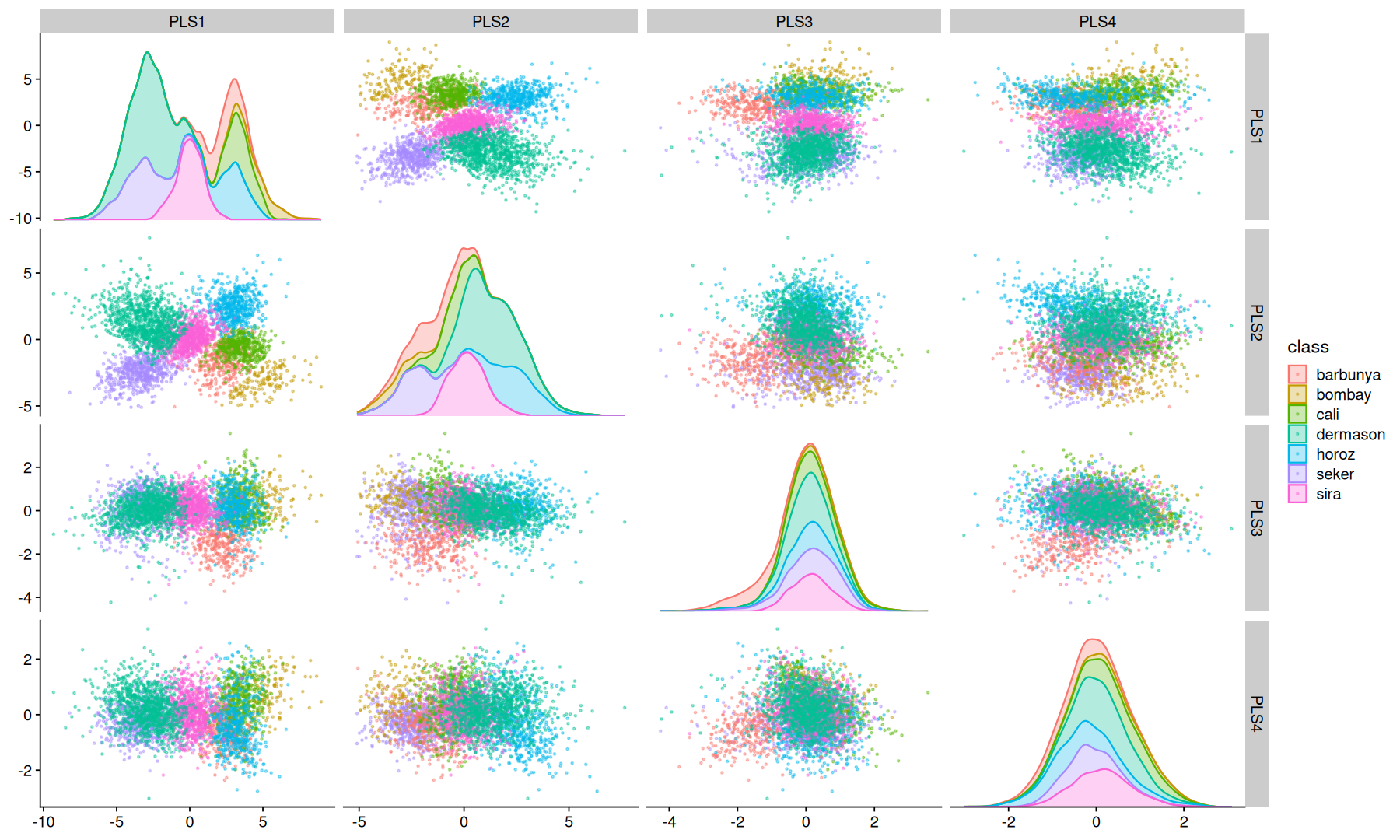
PLS

Partial Least Squares regression is a supervised technique similar to PCA, it finds a linear regression model by projecting the predicted variables and the observable variables to a new space of maximum covariance.

rec |>
step_pls(all_predictors(), outcome='class', num_comp = 4) |>
plot_rec(class, test)

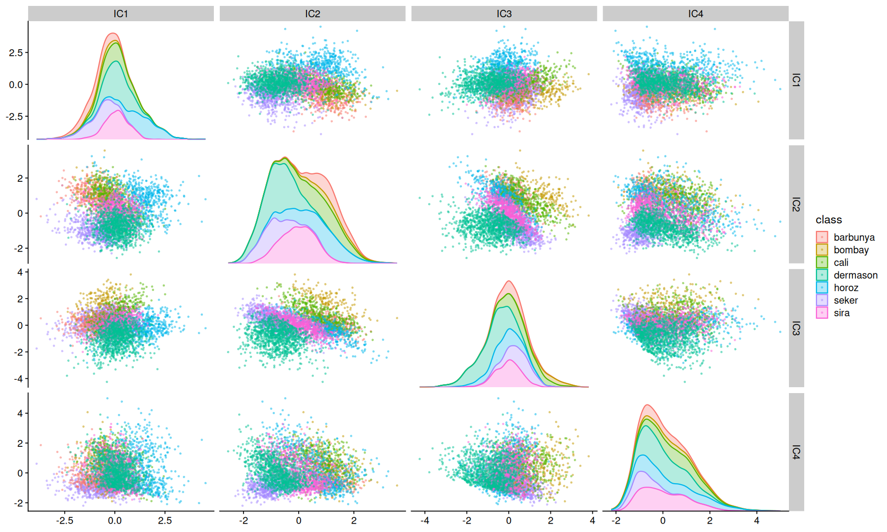
ICA

Independent Component Analysis is a computational method for separating a signal into additive subcomponents. This is done by assuming that at most one subcomponent is Gaussian and that the subcomponents are statistically independent from each other.

rec |>
step_ica(all_predictors(), num_comp = 4) |>
plot_rec(class, test)

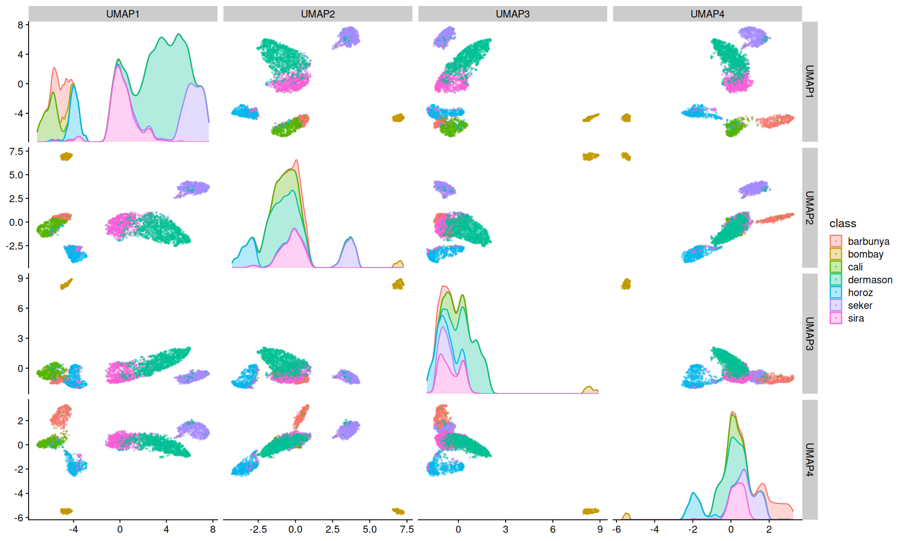
UMAP

Uniform Manifold Approximation and Projection is a dimension reduction technique that can be used for visualisation similarly to t-SNE, but also for general non-linear dimension reduction.

rec |>
step_umap(all_predictors(), num_comp = 4) |>
plot_rec(class, test)

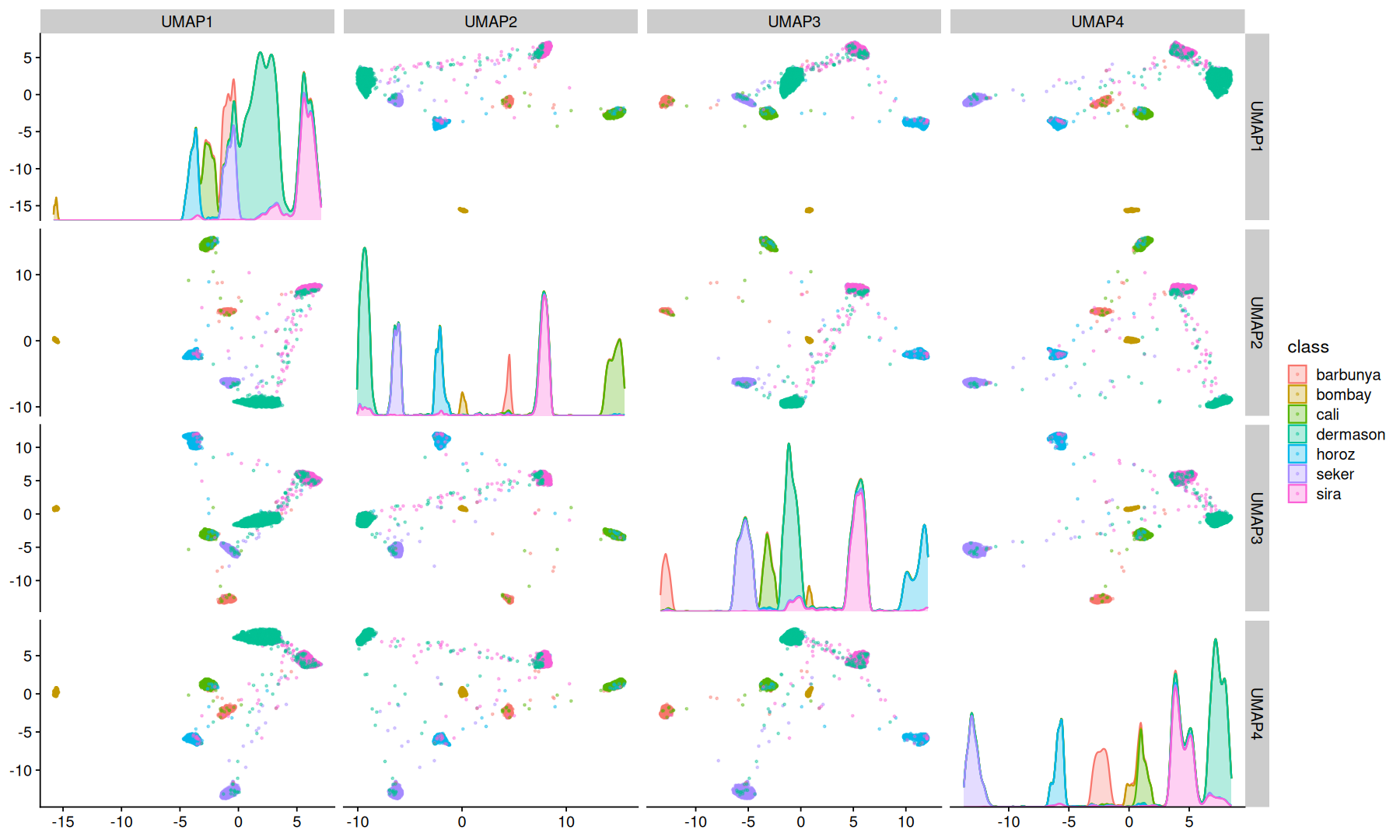
UMAP can also to make use of a label information to perform supervised dimension reduction.

rec |>
step_umap(all_predictors(), outcome=vars(class), num_comp = 4) |>
plot_rec(class, test)

NMF

Non-negative Matrix Factorization is a technique to factorize a matrix V into two matrices W and H, such that W * H = V, with the property that all three matrices have no negative elements.

Note that for demonstration purposes the data was transformed to be within 0 and 1, in practice if your data have negative numbers NMF is not a good fit.

rec |>
# transform data to be non-negative
step_range(all_predictors(), min=0, max=1, clipping = FALSE) |>
step_nnmf_sparse(all_predictors(), num_comp = 4) |>
plot_rec(class, test)

Further reading

https://www.tmwr.org/dimensionality