suppressPackageStartupMessages({
library(tidyverse)
library(cowplot)
library(ggrepel)
library(ggbeeswarm)
library(patchwork)
library(RColorBrewer)
library(pheatmap)
library(broom)
})
theme_set(theme_cowplot())
options(repr.plot.width=15,repr.plot.height=9, width=150)

Crinacle IEMs Ranking

data preprocessing

# data downloaded from the site on 2023-11-17
a <- read_csv("crinacle.csv", col_types='', name_repair = 'universal')

# group signatures into fewer categories
a <- mutate(a, sig_group=case_when(
    grepl("Balanced", Signature) ~ "Neutral",
    Signature == "Mid-centric" ~ "Neutral",
    Signature == "Bassy" ~ "Warm",
    grepl("Dark", Signature) ~ "Warm",
    grepl("Warm", Signature) ~ "Warm",
    grepl("Bright", Signature) ~ "Bright",
    grepl("failure", Signature) ~ "Unique",
    Signature == "Variable" ~ "Unique",
    Signature == "W-shaped" ~ "Unique",
    grepl("U-shape", Signature) ~ "U-shaped",
    grepl("V-shape", Signature) ~ "V-shaped",
    grepl("Neutral with", Signature) ~ "Neutral",
    TRUE ~ Signature
))

rank_levels <- c(
    'N/A', 'DQ', 'F', 'E', 
    'D-', 'D', 'D+',
    'C-', 'C', 'C+',
    'B-', 'B', 'B+',
    'A-', 'A', 'A+',
    'S-', 'S', 'S+'
)

# transform ranks into ordered factors
a <- mutate(a, 
    Rank=ordered(Rank, levels=rank_levels),
    Technical.Grade=ordered(Technical.Grade, levels=rank_levels),
    Tone.Grade=ordered(Tone.Grade, levels=rank_levels),
    Value.Rating=ordered(replace_na(Value.Rating, ''), levels=c('', '★','★★','★★★'))
)

a <- mutate(a,
    # extract brand from model
    brand=str_extract(Model, '^\\S+'),
    # number of total drivers
    n_drivers=unlist(map(str_split(Setup, ' '), ~ sum(as.numeric(replace_na(str_extract(.x, '\\d+'), "1"))))),
    # number of distict drivers
    n_setup=lengths(str_split(Setup, ' ')),
    # group setup into fewer categories
    setup_group=case_when(
        grepl("^\\d+DD$", Setup) ~ "DD",
        grepl("^\\d+BA$", gsub("\\/","",Setup)) ~ "BA",
        grepl("\\?|MS|Piezo|BC|Exciter|AMT", Setup) ~ "Others",
        Setup == 'Electrostatic' ~ 'EST',
        n_setup == 2 ~ "Hybrid",
        n_setup == 3 ~ 'Tribrid',
        TRUE ~ Setup
    )
)

# rename some columns
a <- rename(a,
    Price_MSRP=Pricesort
)

# remove discontinued/free stuff
a <- filter(a, Price_MSRP>0, Price_MSRP<99999)

New names:
• `Value Rating` -> `Value.Rating`
• `Price (MSRP)` -> `Price..MSRP.`
• `Tone Grade` -> `Tone.Grade`
• `Technical Grade` -> `Technical.Grade`

head(a)

A tibble: 6 × 19

Rank	Value.Rating	Model	Price..MSRP.	Signature	Comments	Tone.Grade	Technical.Grade	Setup	Status	Ranksort	Tonesort	Techsort	Price_MSRP	sig_group	brand	n_drivers	n_setup	setup_group
<ord>	<ord>	<chr>	<chr>	<chr>	<chr>	<ord>	<ord>	<chr>	<chr>	<dbl>	<dbl>	<dbl>	<dbl>	<chr>	<chr>	<dbl>	<int>	<chr>
S-	★★	Hidition Viento(B-mode, custom)	950	Variable	Best-in-class tuning and tonal balance with near-perfect coherency. Recommended as a custom-fit.	S+	A+	4BA	Zeppelin & Co demo unit	14	1	13	950	Unique	Hidition	4	1	BA
S-	★★	ThieAudio Monarch Mk2	1000	Neutral with bass boost	NA	S+	A+	2EST 6BA 1DD	Available for demo at The Hangout	14	1	13	1000	Neutral	ThieAudio	9	3	Tribrid
A+	★	Hidition NT6	1050	Neutral	If Etymotic made a multi-BA IEM, this would be the closest to that dream	S-	A+	6BA	Null Audio demo unit	20	7	13	1050	Neutral	Hidition	6	1	BA
A+	★	ThieAudio V16 Divinity	1500	Neutral with bass boost	NA	S-	A+	16BA	Available for demo at The Hangout	20	7	13	1500	Neutral	ThieAudio	16	1	BA
A+	★	Sony IER-Z1R	1700	Mild V-shape	Extended yet natural treble, realistic sub-bass focus and spacious imaging capabilities.	A+	S-	1BA 2DD	Personal unit	20	13	7	1700	V-shaped	Sony	3	2	Hybrid
A+	★★★	Moondrop Variations	520	U-shaped	Sub-bass-focused signature with Moondrop's clean tuning makes this one of the best $500 tribrids.	S	A	2EST 2BA 1DD	Available for demo at The Hangout	24	3	21	520	U-shaped	Moondrop	5	3	Tribrid

Grade Correlations

select(a, Model, Rank, Technical.Grade, Tone.Grade, Value.Rating) |>
pivot_longer(names_to = 'k', values_to = 'v', -c(Model, Value.Rating)) %>%
inner_join(eval(.), by=c('Model', 'Value.Rating'), relationship = "many-to-many") |>
filter(k.x<k.y) |>
mutate(l=paste(k.x, 'x',k.y)) |>
mutate(v=abs(as.numeric(v.x)-as.numeric(v.y))) |>
arrange(Value.Rating) -> b
ggplot(b, aes(x=v.x, y=v.y, color=Value.Rating)) + 
scale_color_manual(values=c('gray','#c7e9c0','#74c476','#006d2c')) +
geom_jitter() + 
facet_wrap(~l) +
labs(x='', y='') +
theme(axis.text.y=element_text(hjust=0)) +
geom_label_repel(data=filter(b, v>7), aes(label=Model), size=4, position=position_jitter(), show.legend = FALSE)

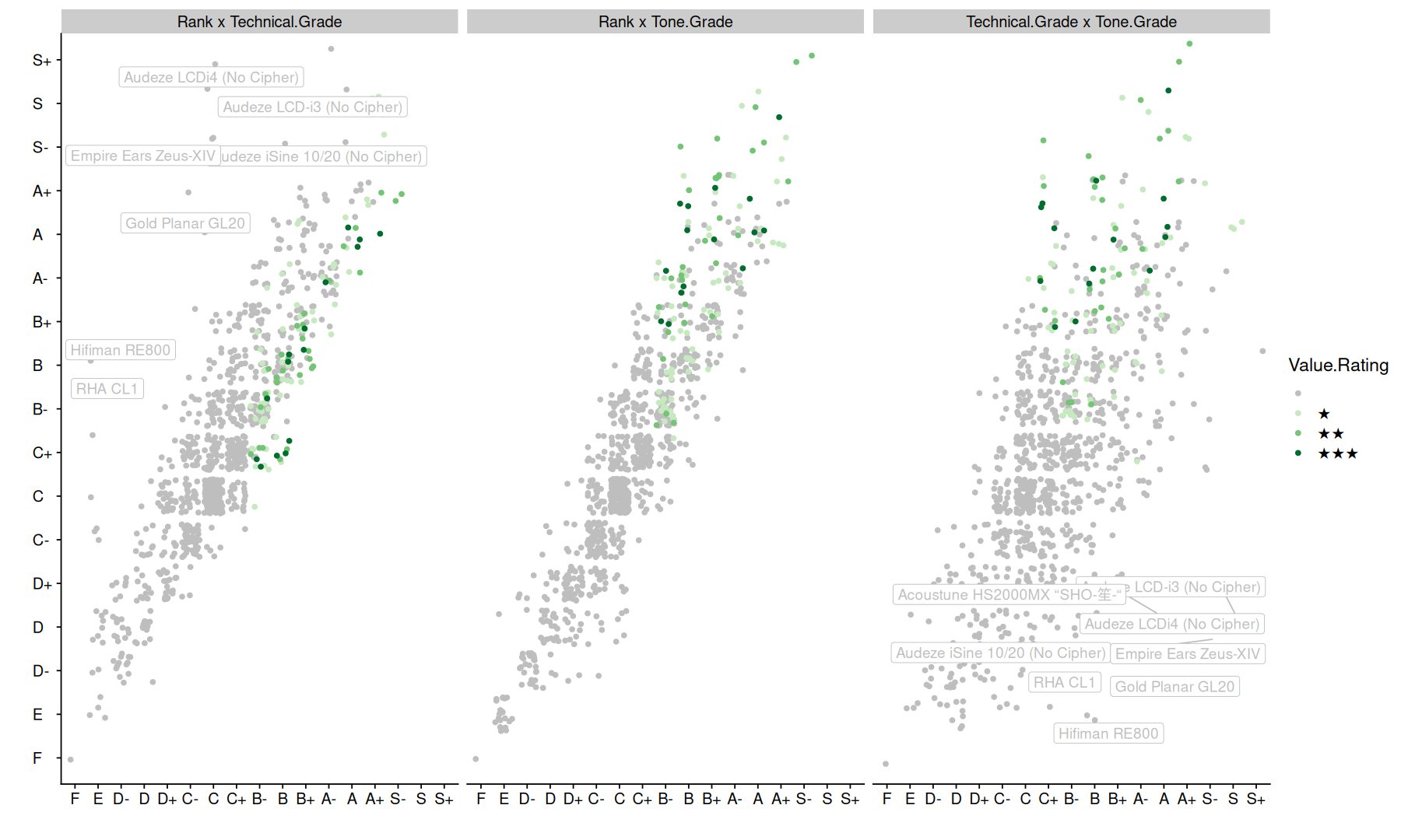
the table includes 3 different grades: Technical, Tone, and overall Rank.

as we can see in the plots, the grades correlate very well with each other, with the exception of a few models labeled in the graph.

with this in mind, in the following analyses, I will focus just on the overall ranking.

Rank distribution

p1 <- ggplot(a, aes(x=Rank, fill=sig_group)) + geom_bar() + coord_cartesian(expand=0)
p2 <- ggplot(a, aes(x=Rank, fill=sig_group)) + geom_bar(position='fill') + labs(y='frequency') + coord_cartesian(expand=0)
p1 + p2 + plot_layout(guides='collect')

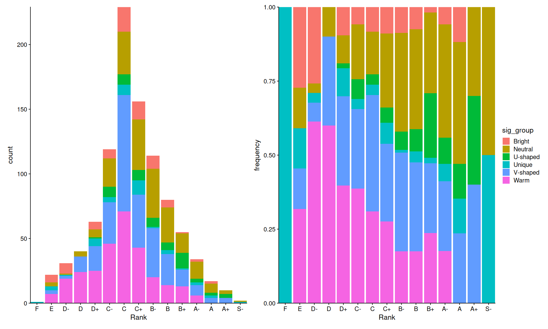
on the left we can see the total amount of headphones by rank, we see a somewhat normally-shaped distribution, with C-Ranks as the most common headphones in the table.

on the right we see the relative frequency of sound signatures by rank, note how warm signatures are frequent at the lower ranks but go down in frequency, while neutral, V-shaped and “unique” signatures dominate the higher ranks.

Price distribution

p1 <- ggplot(a, aes(x=Price_MSRP, fill=Rank)) + 
geom_histogram(bins = 15) + 
scale_x_log10()

p2 <- ggplot(a, aes(y=Rank, x=Price_MSRP)) + 
geom_boxplot() + 
scale_x_log10() + 
geom_quasirandom(alpha=0.8, color='gray') +
geom_vline(xintercept=1000, linetype=2, color='darkblue')

p1 + p2

Orientation inferred to be along y-axis; override with `position_quasirandom(orientation = 'x')`

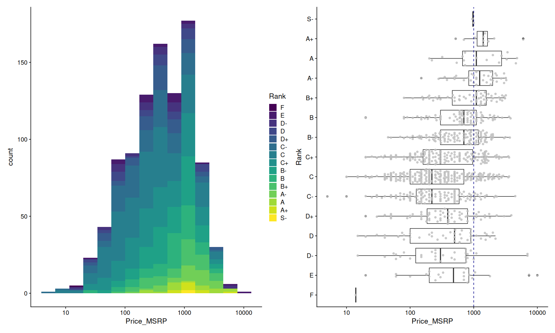
on the left, we can see the overall price distribution of all headphones, note that the x-axes here are log-scaled, we can see headphones for as low as 5 and as high as 10k, but most headphones, are priced around 100~1000.

on the right, we can see the price breakdown by rank, note how even though there is a tendency for higher-ranked headphones to be more expensive you shouldn’t have to spend more than 1k to have the best-sounding headphones.

There still is a lot of variation even among headphones of the same rank, as an example, let’s look at the price variation of rank B headphones:

filter(a, Rank=='B') |> with(summary(Price_MSRP))

   Min. 1st Qu.  Median    Mean 3rd Qu.    Max. 
     20     300     700     896    1100    3800 

even though the median price is 700, you can find headphones at this rank for as low as 20 and as high as 3800 !!

obviously, there is more to the price than just sound, but since this dataset only grades the sonic performance, a natural question that follows is: what is the best price for performance that we can get?

Price x Rank

b <- 
    arrange(a, Price_MSRP) |>
    group_by(Rank) |> 
    mutate(pr=row_number()) |> 
    ungroup() |>
    filter(Rank>="C")

ggplot(b, aes(y=Rank, x=Price_MSRP, color=Value.Rating)) + 
geom_quasirandom() + 
scale_color_hue() +
geom_label_repel(data=filter(b, pr<10), aes(label=Model), min.segment.length = 0, max.overlaps = 20, position = position_quasirandom(), show.legend = FALSE) + 
scale_x_log10()

Orientation inferred to be along y-axis; override with `position_quasirandom(orientation = 'x')`
Orientation inferred to be along y-axis; override with `position_quasirandom(orientation = 'x')`

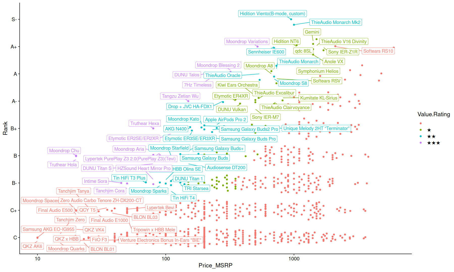
here we have a scatter plot of the Rank x Price, I only included C-Rank and above because I think if you only care about sound performance there is nothing worth the money below this rank.

the top 10 cheapest headphones of each rank are labeled in the graph, and the colors indicate the “Value Rating” from the dataset.

What about TWS ?

filter(b, grepl("Sams|Appl", Model)|grepl("TWS",Comments), pr<10, Price_MSRP>10)

A tibble: 6 × 20

Rank	Value.Rating	Model	Price..MSRP.	Signature	Comments	Tone.Grade	Technical.Grade	Setup	Status	Ranksort	Tonesort	Techsort	Price_MSRP	sig_group	brand	n_drivers	n_setup	setup_group	pr
<ord>	<ord>	<chr>	<chr>	<chr>	<chr>	<ord>	<ord>	<chr>	<chr>	<dbl>	<dbl>	<dbl>	<dbl>	<chr>	<chr>	<dbl>	<int>	<chr>	<int>
B	★★★	Lypertek PurePlay Z3 2.0(PurePlay Z3)(Tevi)	90	Neutral with bass boost	Probably the closest thing to an ER2XR in TWS form.	A	C+	DD	Jaben Melbourne demo unit	112	21	91	90	Neutral	Lypertek	1	1	DD	5
B	★★	Samsung Galaxy Buds	130	Neutral	A surprisingly well-tuned TWS with the technical chops to boot.	A-	B	DD	Personal unit	88	31	57	130	Neutral	Samsung	1	1	DD	7
B	★★	Samsung Galaxy Buds+	150	U-shaped	Tuned even closer to the Harman IE target compared to the original.	B+	B	2DD	Personal unit	100	43	57	150	U-shaped	Samsung	2	1	DD	8
B+	★★	Samsung Galaxy Buds Pro	200	Warm V-shape	More lower mids than your average Harman-tuned IEM, but works in its favour by being more pleasant.	A+	B	2DD	Available for demo at The Hangout	70	13	57	200	Warm	Samsung	2	1	DD	6
B+	★★	Samsung Galaxy Buds2 Pro	230	U-shaped	A less shouty interpretation of Harman with the same controlled yet impactful bass response.	S-	B	2DD	Available for demo at The Hangout	64	7	57	230	U-shaped	Samsung	2	1	DD	8
B+	★★	Apple AirPods Pro 2	250	Mild V-shape	A more exciting sound signature in comparison to its predecessor, with little in terms of drawbacks.	A+	B	DD	Available for demo at The Hangout	70	13	57	250	V-shaped	Apple	1	1	DD	9

Interestingly, some wireless buds make it into the top 10, it’s not the best you can get for the money but it’s up there which I found notable.

Brands

filter(b, Rank>"C", pr<10) |>
add_count(brand, name='total') |>
ggplot(aes(y=fct_reorder(brand, total), fill=Rank)) +
geom_bar(position='stack') +
labs(y="") +
coord_cartesian(expand=0)

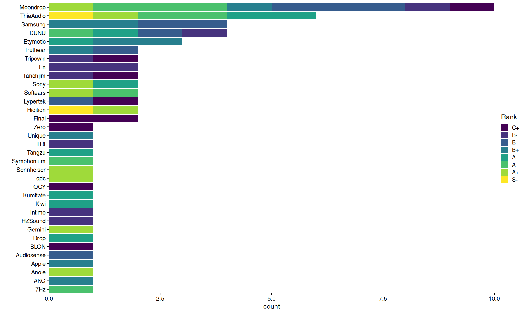
if we group these selected top 10s by brand, we see that Moondrop appears 11 times across the ranks C and above, followed by ThieAudio.

Setup

p1 <- ggplot(a, aes(x=n_setup, y=Price_MSRP, group=n_setup)) + 
geom_boxplot() + 
scale_y_log10()

p2 <- ggplot(a, aes(x=n_drivers, y=Price_MSRP)) + geom_boxplot(aes(group=n_drivers)) + scale_y_log10()

p1+p2

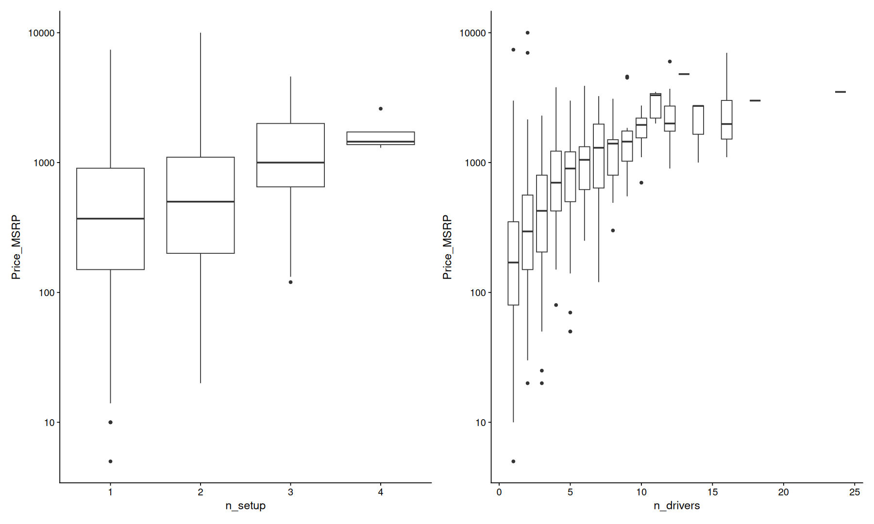
there is a clear correlation between the total number of drivers, drivers setup, and the price, as expected.

p1 <- ggplot(a, aes(x=n_setup, y=Rank)) + geom_boxplot()
p2 <- ggplot(a, aes(x=n_drivers, y=Rank)) + geom_boxplot()

p1+p2

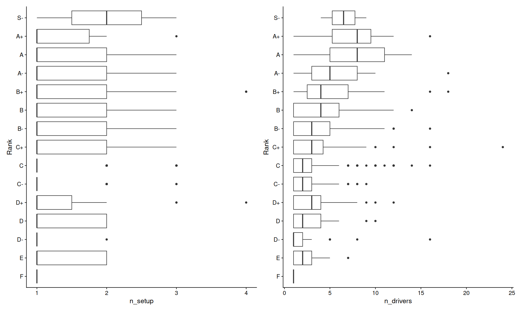
more drivers do not necessarily mean better sound, although highly ranked headphones tend to have more drivers.

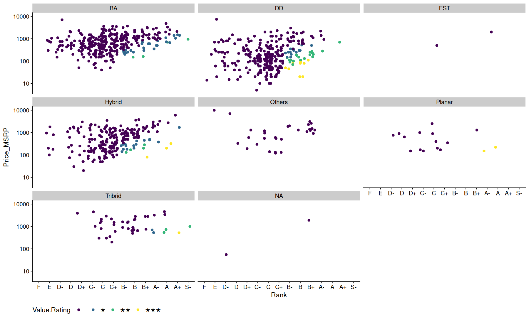
ggplot(a, aes(x=Rank, y=Price_MSRP, color=Value.Rating)) + 
geom_jitter(size=2) +
facet_wrap(~setup_group) +
scale_y_log10() +
theme(legend.position='bottom')

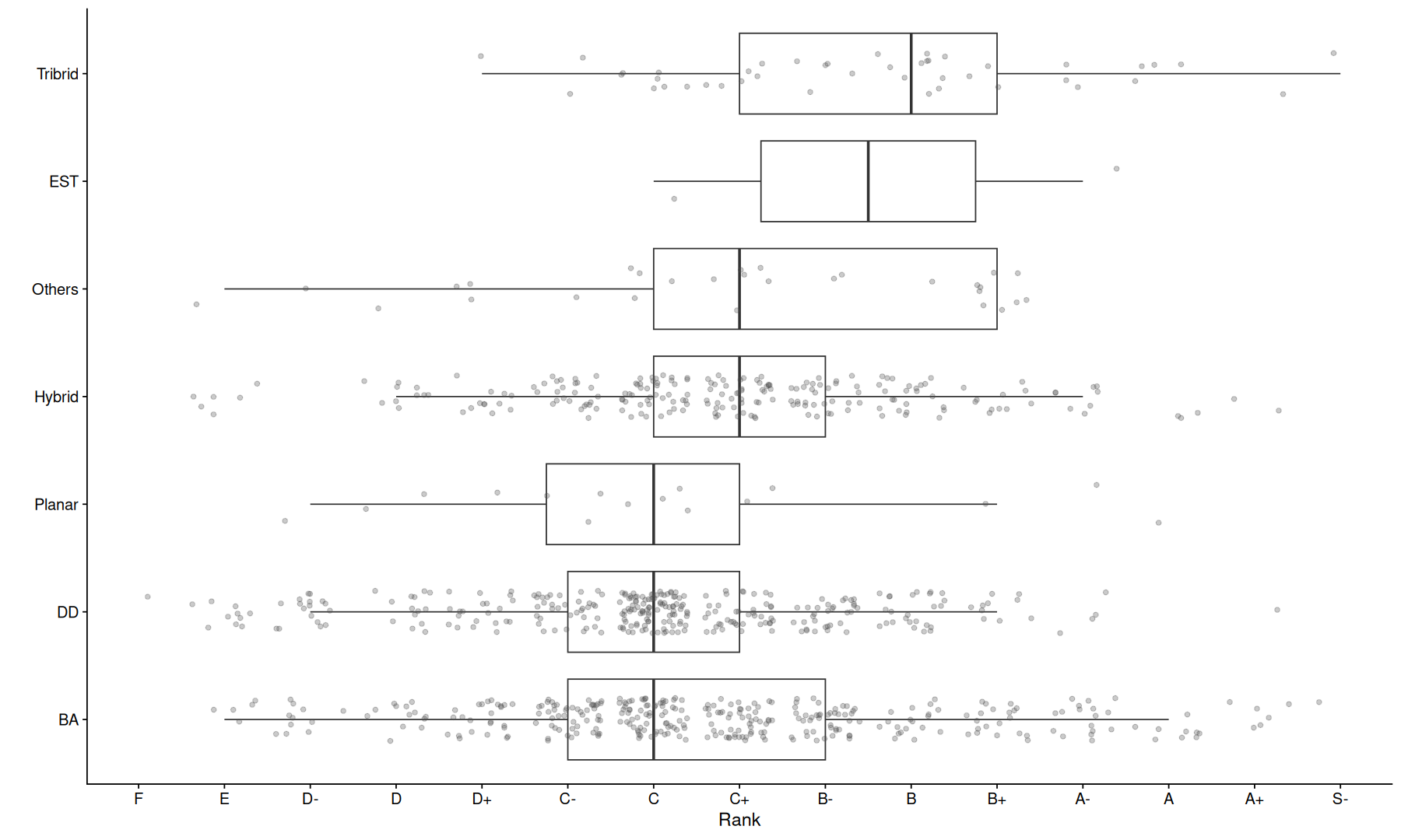
filter(a, !is.na(setup_group)) |>
ggplot(aes(x=Rank, y=fct_reorder(setup_group,as.numeric(Rank)), group=setup_group)) + 
geom_boxplot(outlier.shape = NA) +
geom_jitter(height=0.2,color='gray30',alpha=0.3) +
labs(y="")

Regression model for Rank

mutate(a, 
       n_DD=as.numeric(ifelse(grepl("DD", Setup), replace_na(str_extract(Setup, '(\\d+)DD', group=1), "1"), 0)),
       n_BA=as.numeric(ifelse(grepl("BA", Setup), replace_na(str_extract(Setup, '(\\d+)BA', group=1), "1"), 0)),
       n_EST=as.numeric(ifelse(grepl("EST|Electrostatic", Setup), replace_na(str_extract(Setup, '(\\d+)EST', group=1), "1"), 0)),
       n_planar=as.numeric(ifelse(grepl("Planar", Setup), replace_na(str_extract(Setup, '(\\d+)Planar', group=1), "1"), 0))
) |>
glm(as.numeric(Rank) ~ log(Price_MSRP) + n_drivers + n_setup + n_planar + n_DD + n_EST + n_BA + sig_group + setup_group, data=_, family = 'gaussian') -> m
summary(m)

Call:
glm(formula = as.numeric(Rank) ~ log(Price_MSRP) + n_drivers + 
    n_setup + n_planar + n_DD + n_EST + n_BA + sig_group + setup_group, 
    family = "gaussian", data = mutate(a, n_DD = as.numeric(ifelse(grepl("DD", 
        Setup), replace_na(str_extract(Setup, "(\\d+)DD", group = 1), 
        "1"), 0)), n_BA = as.numeric(ifelse(grepl("BA", Setup), 
        replace_na(str_extract(Setup, "(\\d+)BA", group = 1), 
            "1"), 0)), n_EST = as.numeric(ifelse(grepl("EST|Electrostatic", 
        Setup), replace_na(str_extract(Setup, "(\\d+)EST", group = 1), 
        "1"), 0)), n_planar = as.numeric(ifelse(grepl("Planar", 
        Setup), replace_na(str_extract(Setup, "(\\d+)Planar", 
        group = 1), "1"), 0))))

Coefficients:
                           Estimate       Std. Error  t value   Pr(>|t|)    
(Intercept)         5.0388646194512  0.7059948937889  7.13725 1.8868e-12 ***
log(Price_MSRP)     0.3876471381845  0.0702759023098  5.51607 4.4671e-08 ***
n_drivers          -2.1050299659669  0.5819941972715 -3.61693 0.00031378 ***
n_setup             1.1794861463120  0.4946853124821  2.38432 0.01730591 *  
n_planar            0.6001636438329  0.8015013761459  0.74880 0.45416316    
n_DD                1.5737409820566  0.6235871424272  2.52369 0.01177476 *  
n_EST               2.1732189427560  0.6015507027739  3.61269 0.00031888 ***
n_BA                2.2739762780733  0.5791393801483  3.92647 9.2414e-05 ***
sig_groupNeutral    1.1106529366202  0.2823646301092  3.93340 8.9832e-05 ***
sig_groupU-shaped   1.8555293224095  0.3691330964797  5.02672 5.9594e-07 ***
sig_groupUnique    -0.3763688609290  0.4086378940143 -0.92103 0.35726669    
sig_groupV-shaped   0.7164846781807  0.2681806694116  2.67165 0.00767684 ** 
sig_groupWarm      -0.5816734492416  0.2728846228803 -2.13157 0.03329753 *  
setup_groupDD       0.9183154894721  0.3545251992584  2.59027 0.00973667 ** 
setup_groupEST      1.9803622239615  1.5185396115553  1.30412 0.19250692    
setup_groupHybrid  -0.2931567125193  0.5374543577266 -0.54545 0.58556898    
setup_groupOthers   1.1223559977683  0.9857057289061  1.13863 0.25514316    
setup_groupPlanar   1.8350494465020  0.7869457285812  2.33186 0.01991571 *  
setup_groupTribrid -0.3794302558383  1.0502003203315 -0.36129 0.71796042    
---
Signif. codes:  0 '***' 0.001 '**' 0.01 '*' 0.05 '.' 0.1 ' ' 1

(Dispersion parameter for gaussian family taken to be 4.44009424513967)

    Null deviance: 5705.946446962  on 970  degrees of freedom
Residual deviance: 4226.969721373  on 952  degrees of freedom
  (2 observations deleted due to missingness)
AIC: 4223.836289681

Number of Fisher Scoring iterations: 2

tidy(m) |> 
filter(term!='(Intercept)') |>
ggplot(aes(x=estimate, y=fct_reorder(term, estimate), color=p.value<0.05)) + 
geom_point(size=3) +
geom_errorbar(aes(xmin=estimate-std.error, xmax=estimate+std.error)) +
geom_vline(xintercept=0, linetype=2) +
labs(y='')

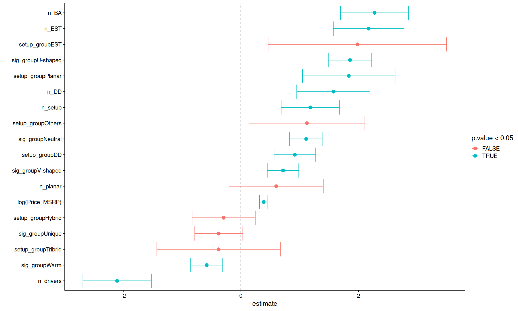
the number of BA, EST, and DD drivers was associated with better ranking but the number of planar drivers did not affect the prediction.

the number of distinct drivers had a positive effect while the total number of drivers was associated with a worst ranking.

Neutral, U-shaped, and V-shaped signatures were associated with better rank while Warm signatures were associated with worse rank.

among different setup groups, Planar, EST, and DD had a positive effect.

price had a small but significant positive effect on ranking.

note however that these interpretations are only valid when the model is utilizing all these variables together, the interpretation could change if we were to add or remove some of these variables.