suppressPackageStartupMessages({
library(recipes)
library(tidyverse)
library(embed)
library(ggforce)
library(tidymodels)
library(mixOmics)
library(fastICA)
library(bestNormalize)
})
theme_set(cowplot::theme_cowplot())
options(repr.plot.width=15,repr.plot.height=9)

Dimensionality Reduction¶

Dataset¶

library(beans)

head(beans)

data_split <- initial_split(beans, prop=0.7, strata=class)

train = training(data_split)
test <- testing(data_split)

table(test$class)


barbunya   bombay     cali dermason    horoz    seker     sira 
     377      149      501     1068      571      616      804

rec <- recipe(class ~ ., data=training(data_split)) |>
step_zv(all_numeric_predictors()) |>
step_orderNorm(all_numeric_predictors()) |>
step_normalize(all_numeric_predictors())

prep(rec) |>
bake(new_data = NULL) |>
head()

plot_rec <- function(recipe, outcome, data) {
    prep(recipe) |>
    bake(new_data = data) |>
    ggplot(aes(x = .panel_x, y = .panel_y, fill={{outcome}}, color={{outcome}})) +
    geom_point(alpha = 0.4, size = 0.5) +
    geom_autodensity(alpha = .3) +
    facet_matrix(vars(-{{outcome}}), layer.diag = 2)
}

PCA¶

Principal Components Analysis is a dimensionality reduction technique to transform data onto a new coordinate system such that the directions (principal components) capture the largest variation in the data.

For a more detailed visualization of PCA results, see PCA Visualization in R

rec |>
step_pca(all_predictors(), num_comp = 4) |>
plot_rec(class, test)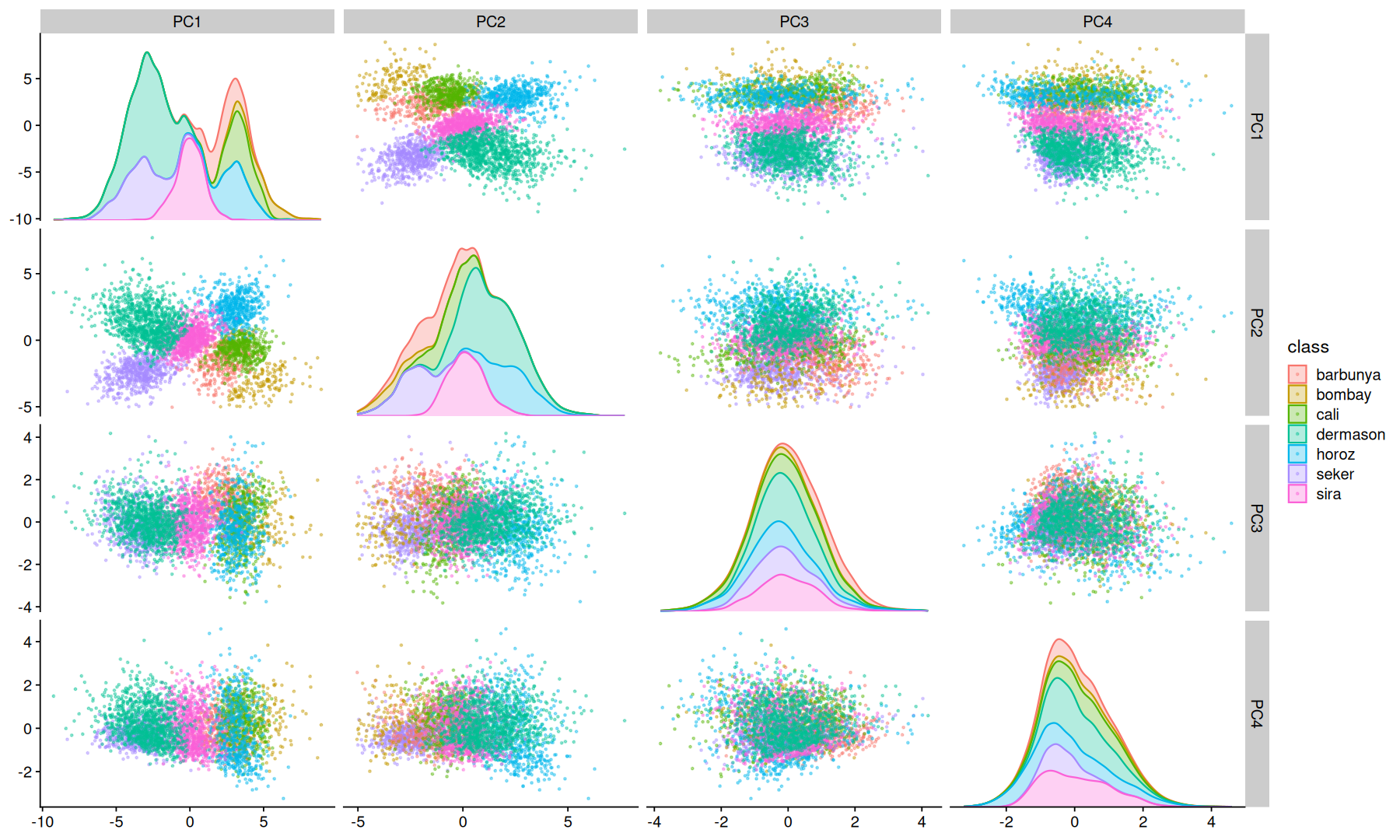

PLS¶

Partial Least Squares regression is a supervised technique similar to PCA, it finds a linear regression model by projecting the predicted variables and the observable variables to a new space of maximum covariance.

rec |>
step_pls(all_predictors(), outcome='class', num_comp = 4) |>
plot_rec(class, test)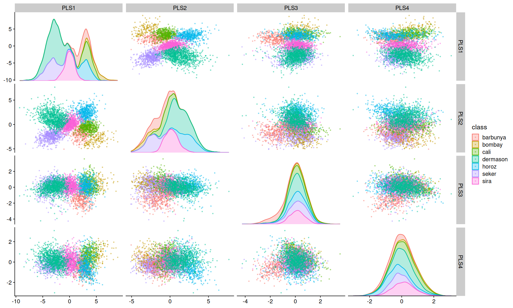

ICA¶

Independent Component Analysis is a computational method for separating a signal into additive subcomponents. This is done by assuming that at most one subcomponent is Gaussian and that the subcomponents are statistically independent from each other.

rec |>
step_ica(all_predictors(), num_comp = 4) |>
plot_rec(class, test)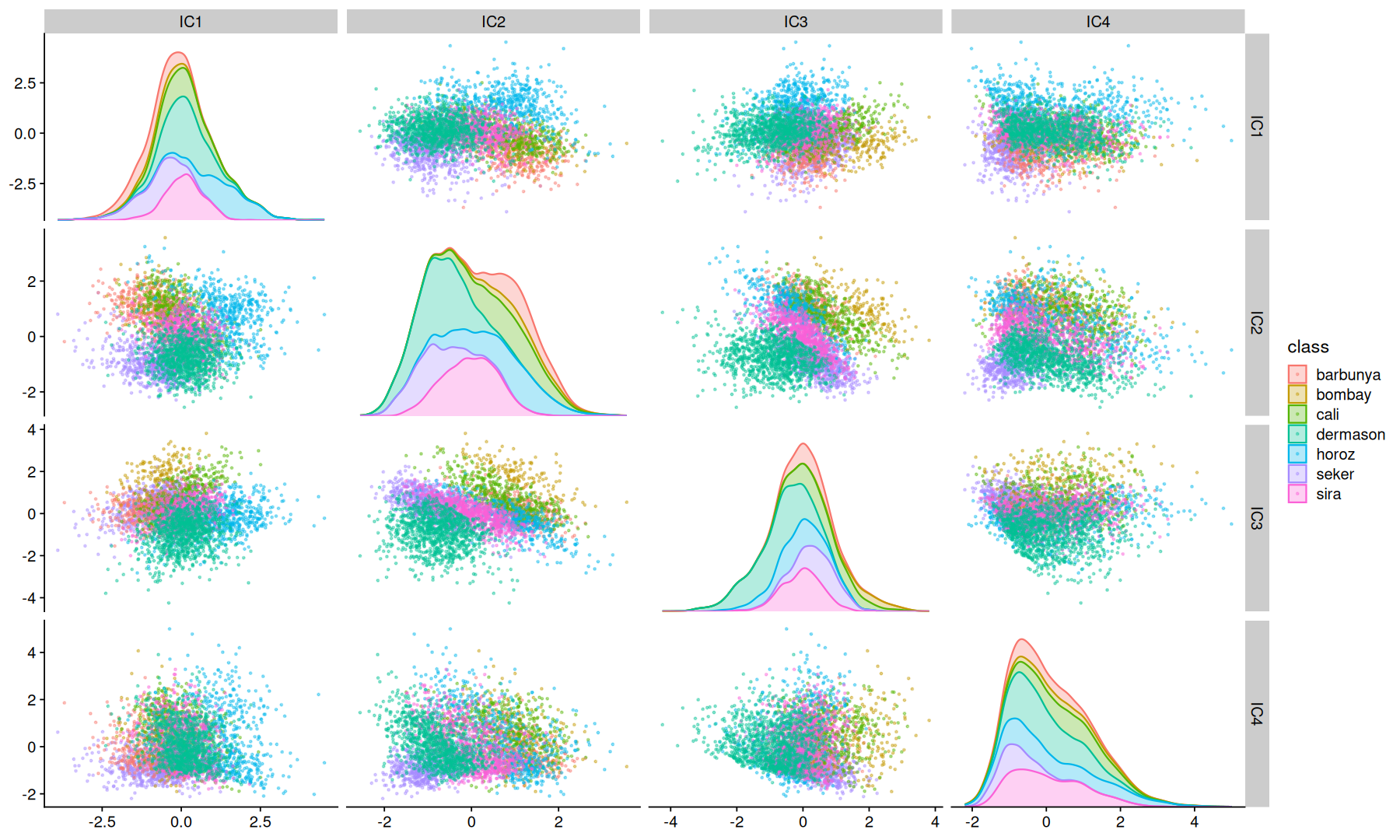

UMAP¶

Uniform Manifold Approximation and Projection is a dimension reduction technique that can be used for visualisation similarly to t-SNE, but also for general non-linear dimension reduction.

rec |>
step_umap(all_predictors(), num_comp = 4) |>
plot_rec(class, test)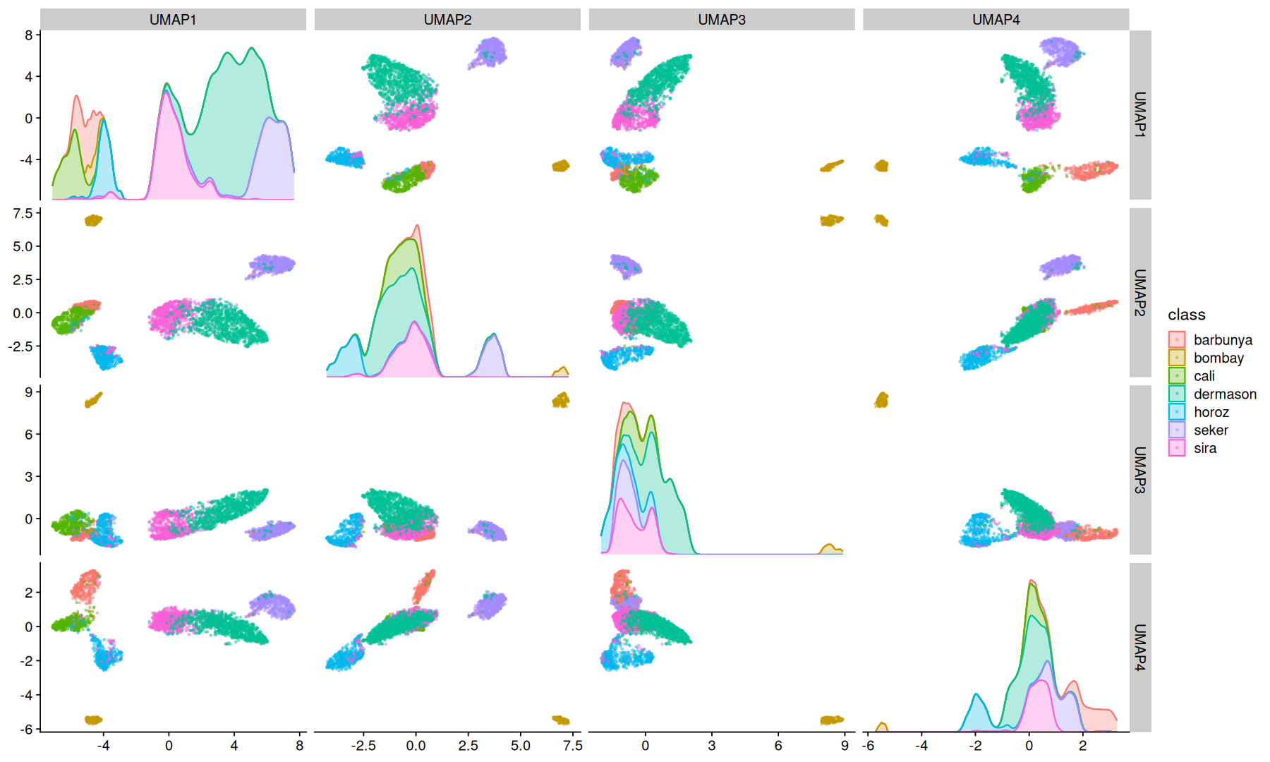

UMAP can also to make use of a label information to perform supervised dimension reduction.

rec |>
step_umap(all_predictors(), outcome=vars(class), num_comp = 4) |>
plot_rec(class, test)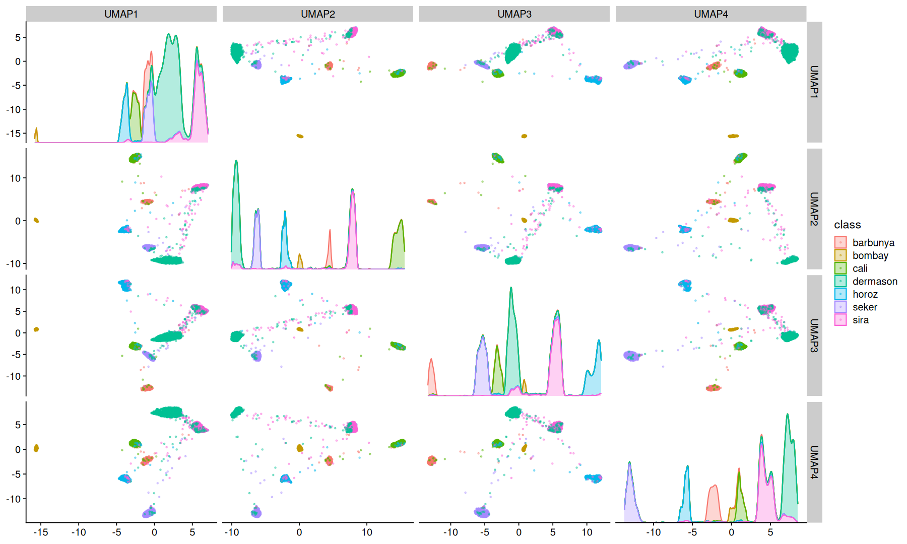

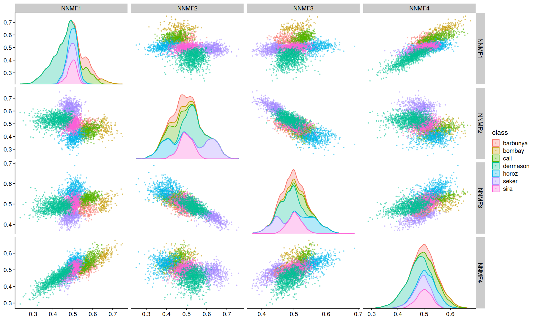
NMF¶

Non-negative Matrix Factorization is a technique to factorize a matrix V into two matrices W and H, such that W * H = V, with the property that all three matrices have no negative elements.

Note that for demonstration purposes the data was transformed to be within 0 and 1, in practice if your data have negative numbers NMF is not a good fit.

rec |>
# transform data to be non-negative
step_range(all_predictors(), min=0, max=1, clipping = FALSE) |>
step_nnmf_sparse(all_predictors(), num_comp = 4) |>
plot_rec(class, test)

Dimensionality Reduction