suppressPackageStartupMessages({
library(tidyverse)
library(cowplot)
library(ggrepel)
library(pheatmap)
library(viridis)
library(matrixStats)
})
theme_set(theme_cowplot())
options(repr.plot.width=15,repr.plot.height=9)

Mahjong Yaku stats¶

Analysis of yaku stats using Tenhou winning hands data, downloaded in may 2023

the data¶

read_tsv("data/data.tsv.gz", col_types="") %>%
select(-hanp, -chanp, -rate) %>% 
complete(yaku, nesting(month, year, room, mode, total)) %>% 
mutate(count=ifelse(is.na(count), 0, count)) %>%
mutate(date=as.Date(paste0(year,'-',month,'-01'))) %>%
inner_join(read_tsv("data/rooms.tsv", col_types=""), by="room") %>%
inner_join(read_tsv("data/yakus.tsv", col_types=""), by='yaku') %>%
inner_join(read_tsv("data/modes.tsv", col_types=""), by='mode') %>%
mutate(yaku_romaji=str_to_title(yaku_romaji)) %>%
mutate(
    han_value_closed=case_when(
        grepl("yakuman", han_value_closed) ~ str_to_title(han_value_closed),
        TRUE ~ paste(han_value_closed, "Han")
    )
) %>%
mutate(
    han_value_closed=ordered(han_value_closed, levels=c("1 Han", "2 Han", "3 Han", "6 Han", "Yakuman", "Double Yakuman"))
) -> a
head(a)

select(a, year, month, room, mode, total) %>% unique() %>% with(sum(total))

the data contains frequency of yakus in all winning hands played on tenhou since 2007
the data is aggregated by month, room rank and game type, totalling 1.4 billion winning hands

select(a, date, room, mode, total, n_players, n_rounds) %>% unique() %>%
group_by(date) %>% 
summarize(total=sum(total)) -> z1
filter(z1, date %in% c("2009-07-01","2016-11-01","2020-05-01")) -> z1sel
ggplot(z1,aes(x=date, y=total)) + 
geom_line() + 
scale_y_continuous(labels=scales::comma_format()) +
labs(y="total of winning hands per month", x="") +
geom_label_repel(data=z1sel, aes(label=format(date,"%Y-%b")), max.overlaps = Inf, min.segment.length = 0, segment.linetype=2)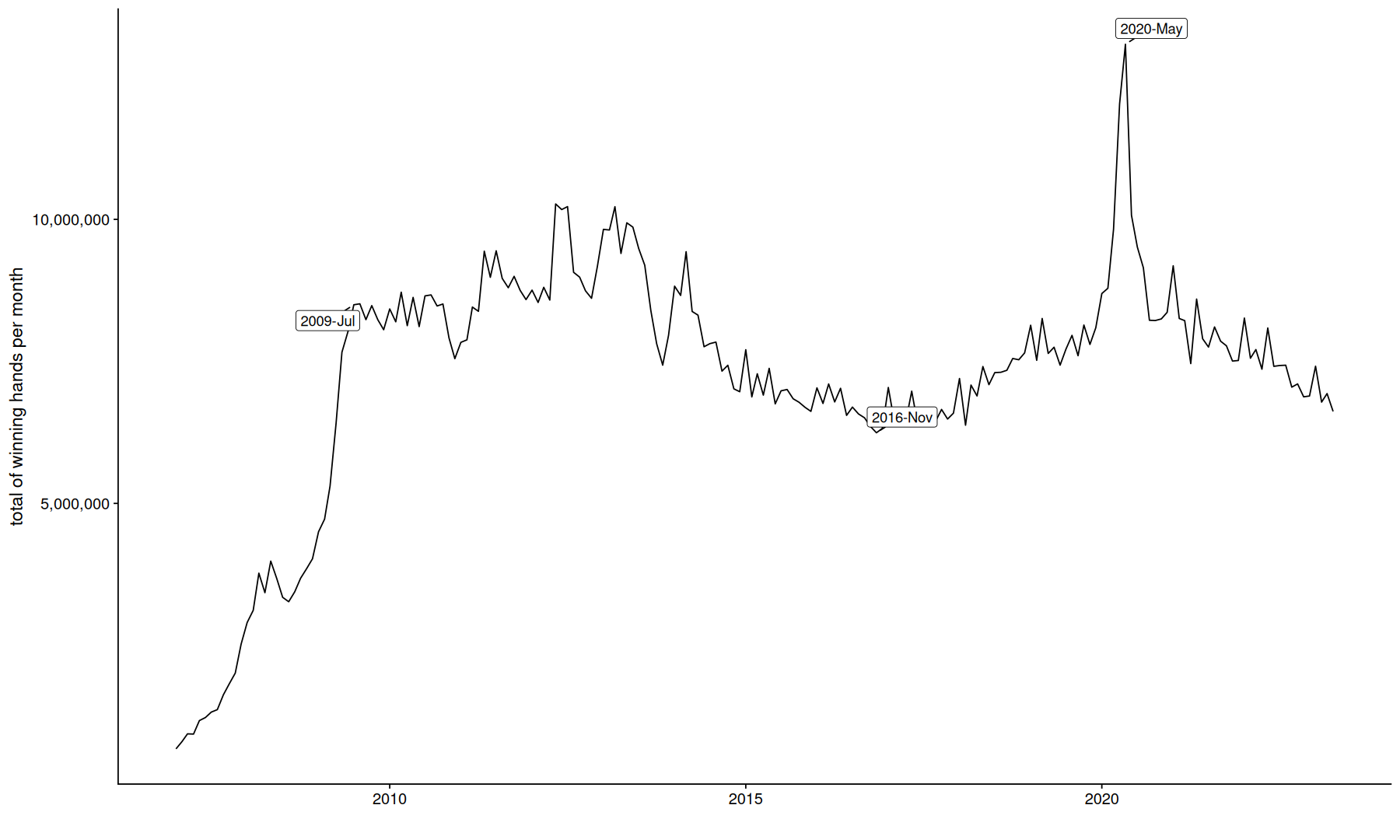

may-2020 had the highest number of winning hands, and is probably because a state of emergency was declared in Japan at the time due to covid-19

game modes popularity over time¶

select(a, date, room, mode, total, n_players, n_rounds) %>% 
mutate(total_p=total/n_rounds) %>%
unique -> z1
group_by(z1, mode, room) %>% slice_max(date) -> z1max
ggplot(z1, aes(x=date, y=total_p, color=mode)) + 
geom_line() + 
scale_y_continuous(labels=scales::comma_format()) + 
geom_text_repel(data=z1max,aes(label=mode), segment.color='gray40', hjust='right', nudge_x=1000, max.iter = 1e4, min.segment.length = 0, box.padding = 0.4) +
facet_wrap(~room, scales="free_y") +
labs(y="# of winning hands / # of rounds",x="") + guides(color='none')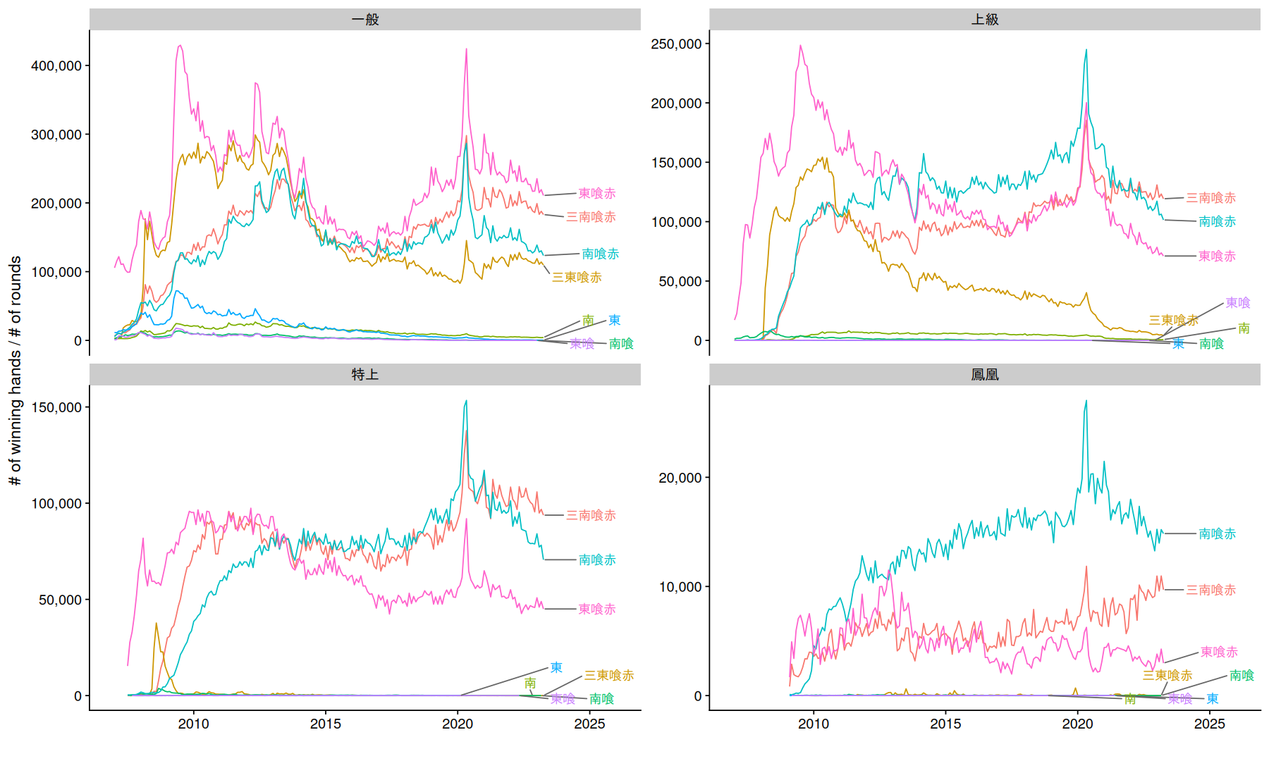

modes without kuitan or akadora are the least popular option
sanma east games are popular on ippan but on a decline in joukyuu, and inexistent in later rooms
sanma south seems to be getting more popular in houou rooms

yaku frequencies vs. han value¶

filter(a, mode=='南喰赤', yaku_romaji!='Bakaze Pei') %>%
group_by(yaku_romaji, han_value_closed) %>% 
summarize(count=sum(count), total=sum(total)) %>%
mutate(p=count/total) %>% arrange(-p) %>%
ggplot(aes(x=han_value_closed, y=p)) +
geom_point(size=2) + 
geom_label_repel(aes(label=yaku_romaji), min.segment.length = 0, max.iter = 1e4, max.overlaps = Inf, box.padding = 0.4) +
scale_y_log10(labels=scales::percent_format(), n.breaks=10) +
theme_bw() +
labs(y="", x="")

`summarise()` has grouped output by 'yaku_romaji'. You can override using the `.groups` argument.

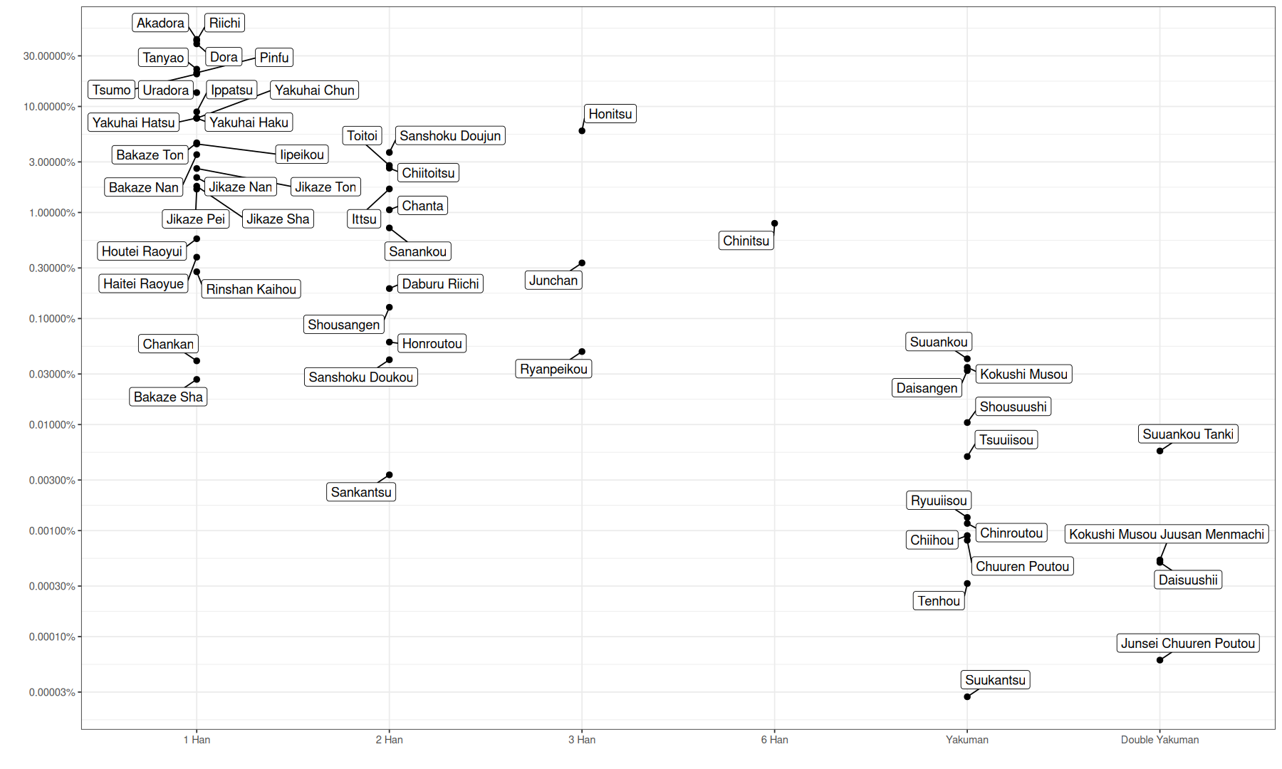
the Y-axis is in log scale, the difference between one tick and the next is 3x
sankantsu is rarer than some yakumans, suukantsu is the rarest yaku at about 1 in 3 millon winning hands
the frequency of the yaku doesn’t quite match its value, an explanation for this could be that players will tend to favor easier and/or more valuable yakus

yaku frequencies over time¶

filter(a, mode=='南喰赤', year>2011) %>% 
mutate(rm=paste(room,mode)) %>%
ggplot(aes(x=date, y=count/total, color=room)) + 
scale_y_continuous(labels=scales::percent_format()) +
geom_smooth(se=FALSE, linewidth=0.5, span=0.3) +
labs(y="",x="") +
scale_x_date(date_labels = "%Y", breaks=as.Date(c("2012-01-01","2017-01-01","2022-01-01"))) +
facet_wrap(~yaku_romaji, scales="free_y") +
theme(
    strip.text = element_text(size = 6), 
    axis.text.y=element_text(size=8),
    axis.text.x=element_text(size=8))

`geom_smooth()` using method = 'loess' and formula = 'y ~ x'

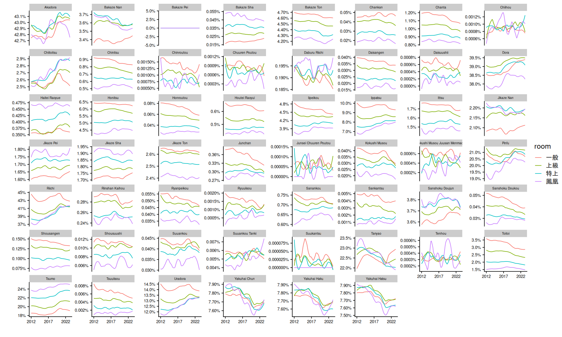
remember this is % of winning hands, the yaku chance is not changing, what changes is the way people play
bakaze pei is weird, its super rare yes, but after 2010 it was never recorded, probably a change in the algorithm avoids a north round extension
I removed the early years because to low amount of data makes it hard to observe the low frequencies of the rarer yakus

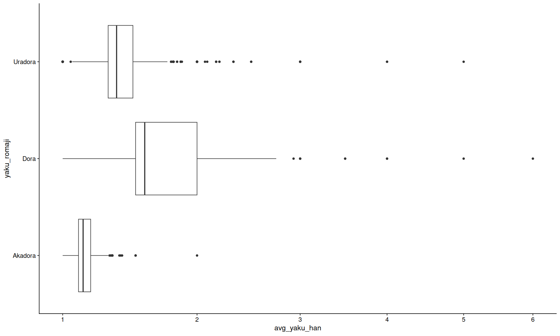
average han value per yaku¶

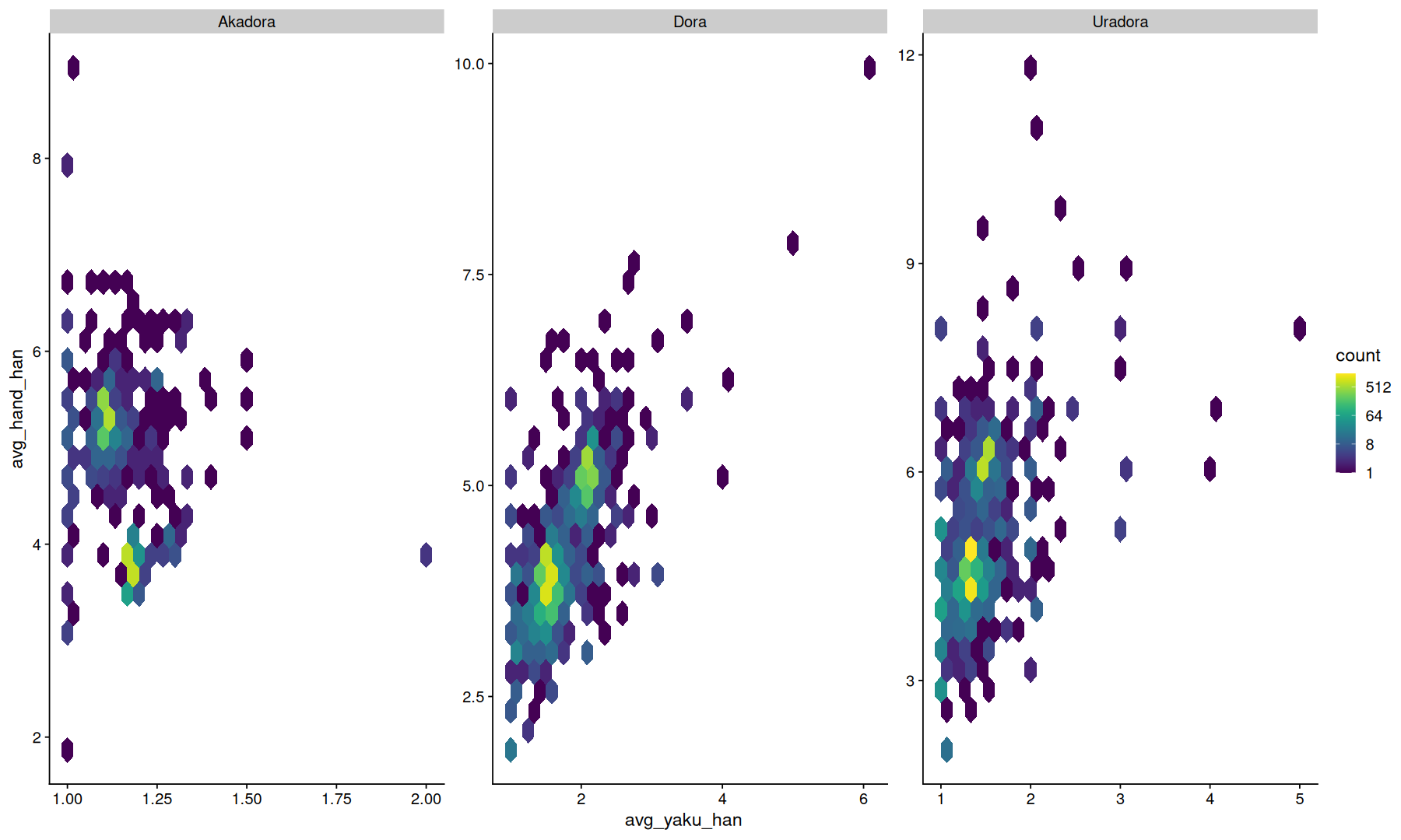
doras can appear more than once on the hand, so we can look at the average amount of value contributed to the hand

select(a, yaku_romaji, avg_yaku_han, avg_hand_han, han_value_closed) %>% unique %>%
filter(yaku_romaji %in% c("Dora", "Akadora", "Uradora")) %>%
ggplot(aes(x=avg_yaku_han, y=yaku_romaji)) + geom_boxplot() + scale_x_sqrt()

Warning message:
"Removed 3 rows containing non-finite values (`stat_boxplot()`)."

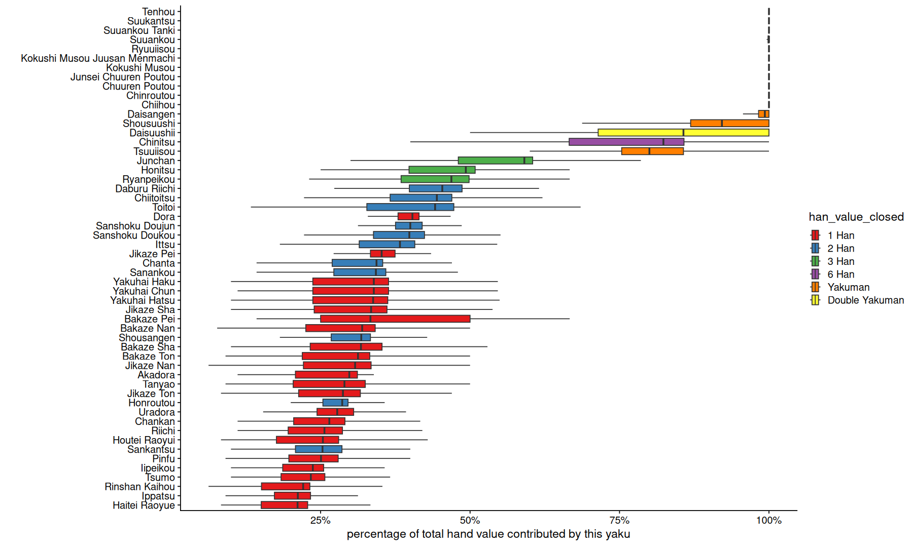
select(a, yaku_romaji, avg_yaku_han, avg_hand_han, han_value_closed, date, room, mode) %>% unique %>%
mutate(perc_han=avg_yaku_han/avg_hand_han) %>%
ggplot(aes(x=perc_han, y=fct_reorder(yaku_romaji, perc_han, .na_rm=TRUE), fill=han_value_closed)) + 
geom_boxplot(outlier.shape = NA) + 
scale_fill_brewer(palette='Set1') +
scale_x_continuous(labels=scales::percent_format()) +
labs(y="", x="percentage of total hand value contributed by this yaku")

Warning message:
"Removed 70864 rows containing non-finite values (`stat_boxplot()`)."

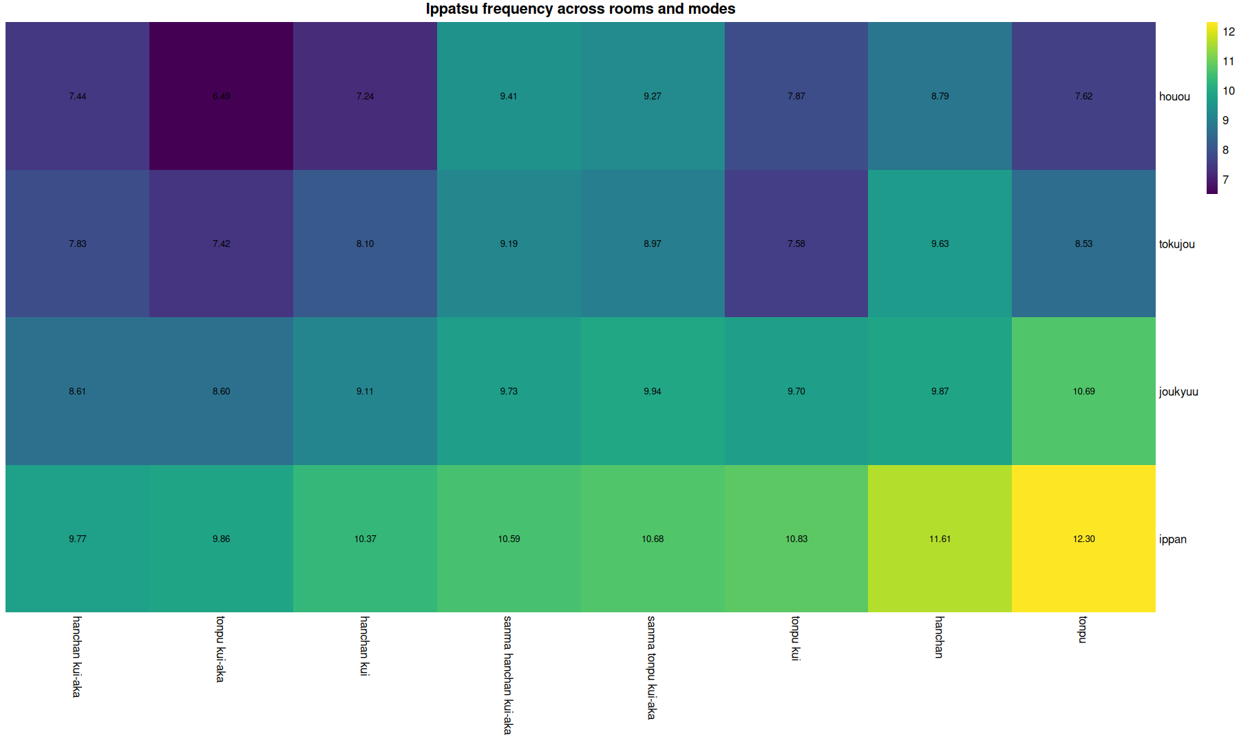
looking at specific yakus¶

filter(a, yaku_romaji=='Ippatsu') %>%
group_by(room_romaji, mode_romaji) %>%
summarize(total=sum(total), count=sum(count)) %>%
mutate(p=100*count/total, total=NULL, count=NULL) %>%
mutate(room_romaji=ordered(room_romaji, levels=c("ippan", "joukyuu", "tokujou", "houou"))) %>%
pivot_wider(names_from = 'mode_romaji', values_from = 'p') %>%
arrange(room_romaji) %>%
column_to_rownames('room_romaji') %>% 
as.matrix() %>%
.[order(rowMaxs(.)),order(colMaxs(.))] %>%
pheatmap(display_numbers = TRUE,main='Ippatsu frequency across rooms and modes', color=viridis(100), number_color = 'black', cluster_rows=F, cluster_cols=F, border_color = NA)

`summarise()` has grouped output by 'room_romaji'. You can override using the `.groups` argument.

filter(a, yaku_romaji=='Tsumo') %>%
group_by(room_romaji, mode_romaji) %>%
summarize(total=sum(total), count=sum(count)) %>%
mutate(p=100*count/total, total=NULL, count=NULL) %>%
pivot_wider(names_from = 'mode_romaji', values_from = 'p') %>%
column_to_rownames('room_romaji') %>% 
as.matrix() %>%
.[order(rowMaxs(.)),order(colMaxs(.))] %>%
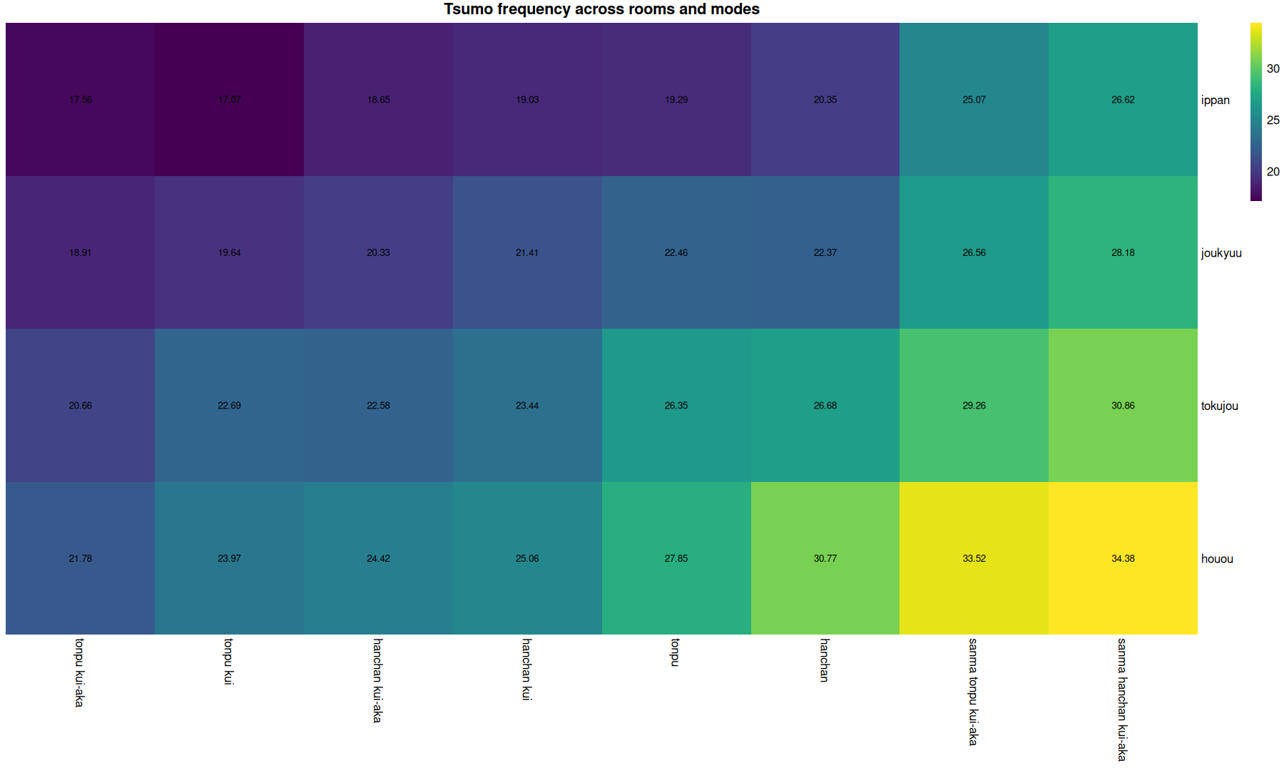
pheatmap(display_numbers = TRUE,main='Tsumo frequency across rooms and modes', color=viridis(100), number_color = 'black', cluster_rows=F, cluster_cols=FALSE, border_color = NA)

`summarise()` has grouped output by 'room_romaji'. You can override using the `.groups` argument.

etc¶

filter(a, avg_yaku_han>4, yaku_romaji=='Dora')

filter(a, yaku_romaji %in% c("Dora", "Akadora", "Uradora")) %>%
ggplot(aes(x=avg_yaku_han, y=avg_hand_han)) + geom_hex() +
scale_fill_viridis(trans='log2') + facet_wrap(~yaku_romaji, scales="free")

Warning message:
"Removed 2269 rows containing non-finite values (`stat_binhex()`)."

mutate(a, z=count/total * avg_yaku_han) %>% filter(total>10000) %>%
select(yaku_romaji, count, total, avg_yaku_han, avg_hand_han, date, room, mode, z) %>% unique

select(a, yaku_romaji, count, total, avg_yaku_han, avg_hand_han, date, room, mode) %>% unique %>%
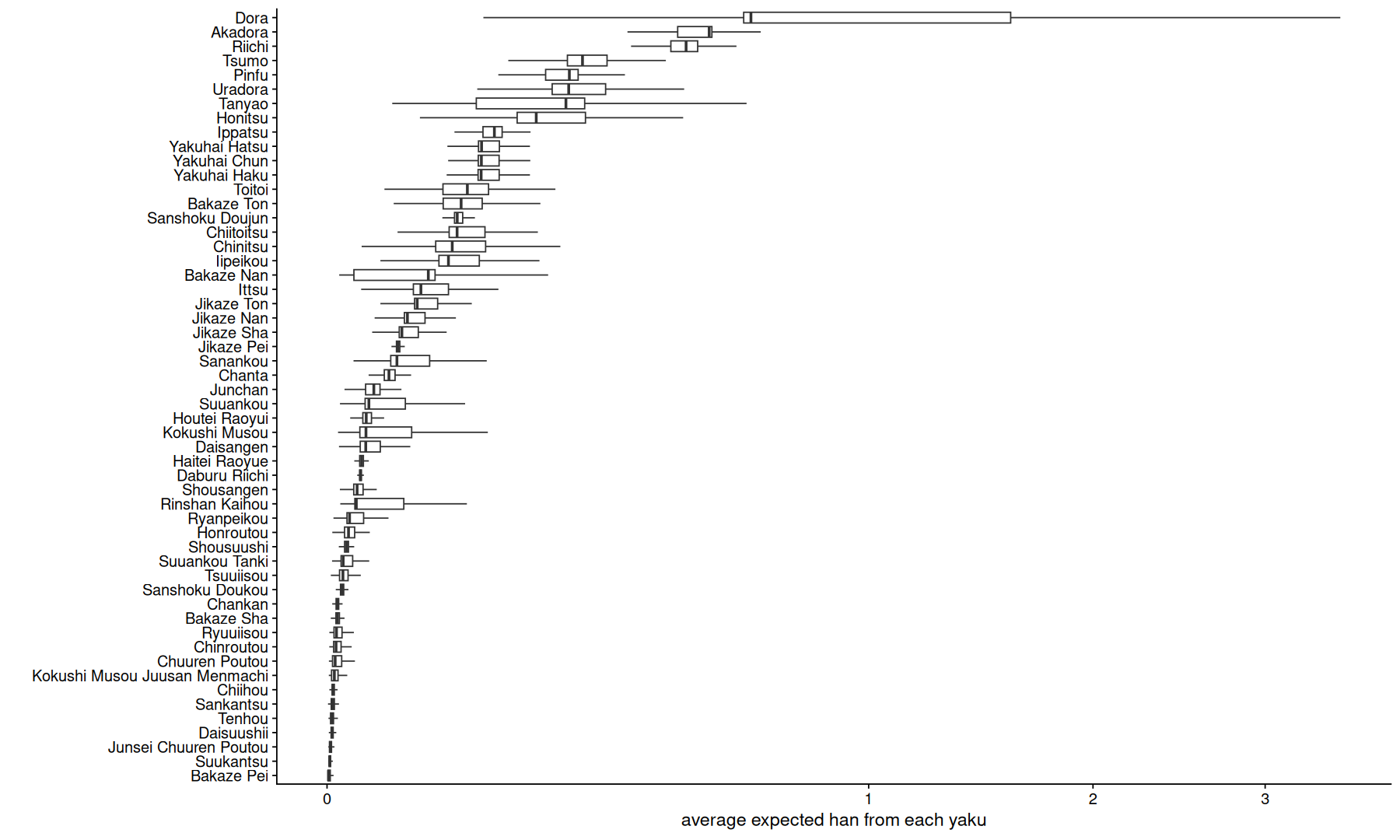
mutate(avg_exp_han=count/total * avg_yaku_han) %>%
ggplot(aes(x=avg_exp_han, y=fct_reorder(yaku_romaji,avg_exp_han, .na_rm=TRUE))) + geom_boxplot(outlier.shape = NA) + 
scale_x_sqrt() +
labs(y="", x="average expected han from each yaku")

Warning message:
"Removed 70864 rows containing non-finite values (`stat_boxplot()`)."

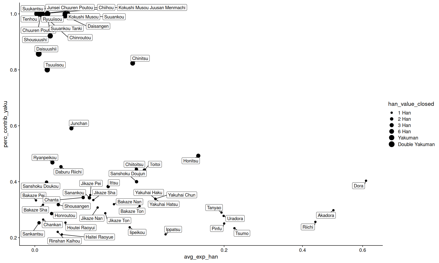
select(a, yaku_romaji, count, total, avg_yaku_han, avg_hand_han, date, room, mode, han_value_closed) %>% unique %>%
mutate(avg_exp_han=count/total * avg_yaku_han, perc_contrib_yaku=avg_yaku_han/avg_hand_han) %>%
group_by(yaku_romaji, han_value_closed) %>%
summarize(
    avg_exp_han=median(avg_exp_han, na.rm=TRUE),
    perc_contrib_yaku=median(perc_contrib_yaku, na.rm=TRUE)
) %>%
ggplot(aes(x=avg_exp_han, y=perc_contrib_yaku)) + 
geom_point(aes(size=han_value_closed)) +
geom_label_repel(aes(label=yaku_romaji), max.overlaps = Inf, min.segment.length = 0) + 
scale_x_sqrt()

`summarise()` has grouped output by 'yaku_romaji'. You can override using the `.groups` argument.