suppressPackageStartupMessages({
    library(tidyverse)
    library(cowplot)
    library(patchwork)
    library(colors3d)
    library(prismatic)
    library(pals)
    theme_set(theme_cowplot())
})
options(repr.plot.width=16,repr.plot.height=10)
Bivariate Color Palette
code
map_to_color2d <- function(data, xvar, yvar, colors=c("yellow", "green", "blue", "magenta"), xtrans="rank", ytrans="rank", size=5, na.color='white') {
    data |>
    summarize(
        min_x = min({{xvar}},na.rm=T), max_x = max({{xvar}},na.rm=T),
        min_y = min({{yvar}},na.rm=T), max_y = max({{yvar}},na.rm=T)
    ) |>
    with(expand_grid(
        x = seq(min_x, max_x, length.out = size),
        y = seq(min_y, max_y, length.out = size)
    )) |>
    mutate(
        color = colors2d(tibble(x,y), xtrans = xtrans, ytrans = ytrans, colors=colors)
    ) |>
    ggplot(aes(x,y,fill=color)) +
    geom_raster() +
    scale_fill_identity() +
    labs(x=as_label(enquo(xvar)), y=as_label(enquo(yvar))) +
    coord_cartesian(expand=0) -> lgd

    data2 <-
    select(data, {{xvar}}, {{yvar}}) |>
    colors2d(xtrans = xtrans, ytrans = ytrans, colors=colors) |>
    bind_cols(data, color=_) |>
    mutate(color=ifelse(is.na({{xvar}}) | is.na({{yvar}}), na.color, color))

    list(data=data2, legend=lgd)
}example
head(iris,3)Loading...
colors <- c('purple', 'blue', 'black', 'red')

r <- map_to_color2d(iris, xvar=Sepal.Length, yvar=Sepal.Width, colors=colors)

ggplot(r$data, aes(y=Petal.Length, x=Petal.Width, color=color, shape=Species, group=Species)) +
stat_ellipse(color='darkgray') +
geom_point(size=3) +
scale_color_identity() +
guides(custom = guide_custom(as_grob(r$legend), width=unit(0.4,'npc'), height=unit(0.4,'npc')))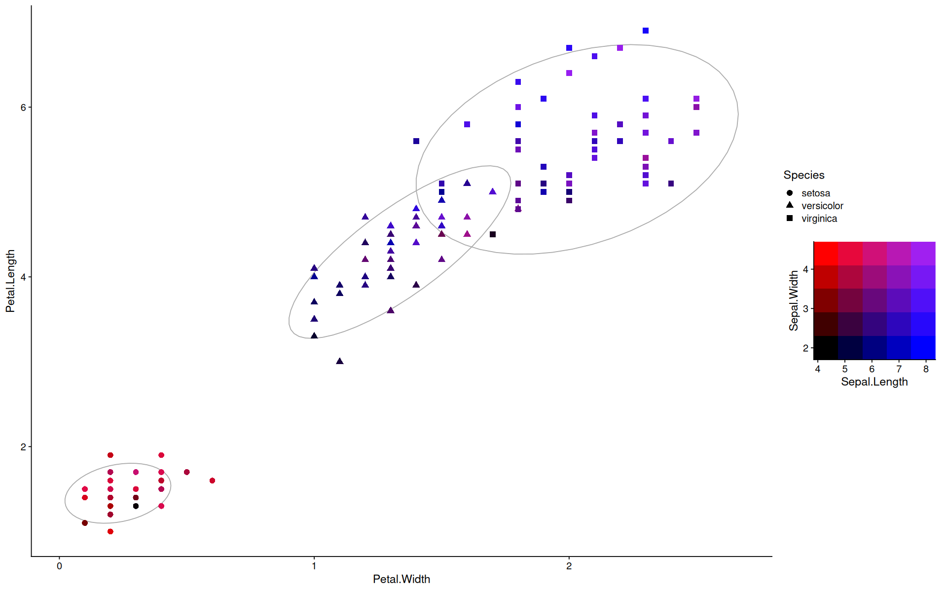
other palettes
color(arc.bluepink())<colors>
#FFFFFFFF #FFE6FEFF #FFBDFFFF #FF80FEFF #E7FFFFFF #D7DAFDFF #D8A6FFFF #C065FEFF #C0FCFDFF #A7CAFFFF #8D7EFDFF #7F65FEFF #74FEFFFF #64C0FFFF #5873FEFF #4B4CFFFF color(arc.bluepink()[c(16,4,1,13)])<colors>
#4B4CFFFF #FF80FEFF #FFFFFFFF #74FEFFFF r <- map_to_color2d(iris, xvar=Sepal.Length, yvar=Sepal.Width, colors=arc.bluepink()[c(16,4,1,13)], size=4)
ggplot(r$data, aes(y=Petal.Length, x=Petal.Width, color=color, shape=Species, group=Species)) +
stat_ellipse(color='darkgray') +
geom_point(size=3) +
scale_color_identity() +
guides(custom = guide_custom(as_grob(r$legend), width=unit(0.4,'npc'), height=unit(0.4,'npc')))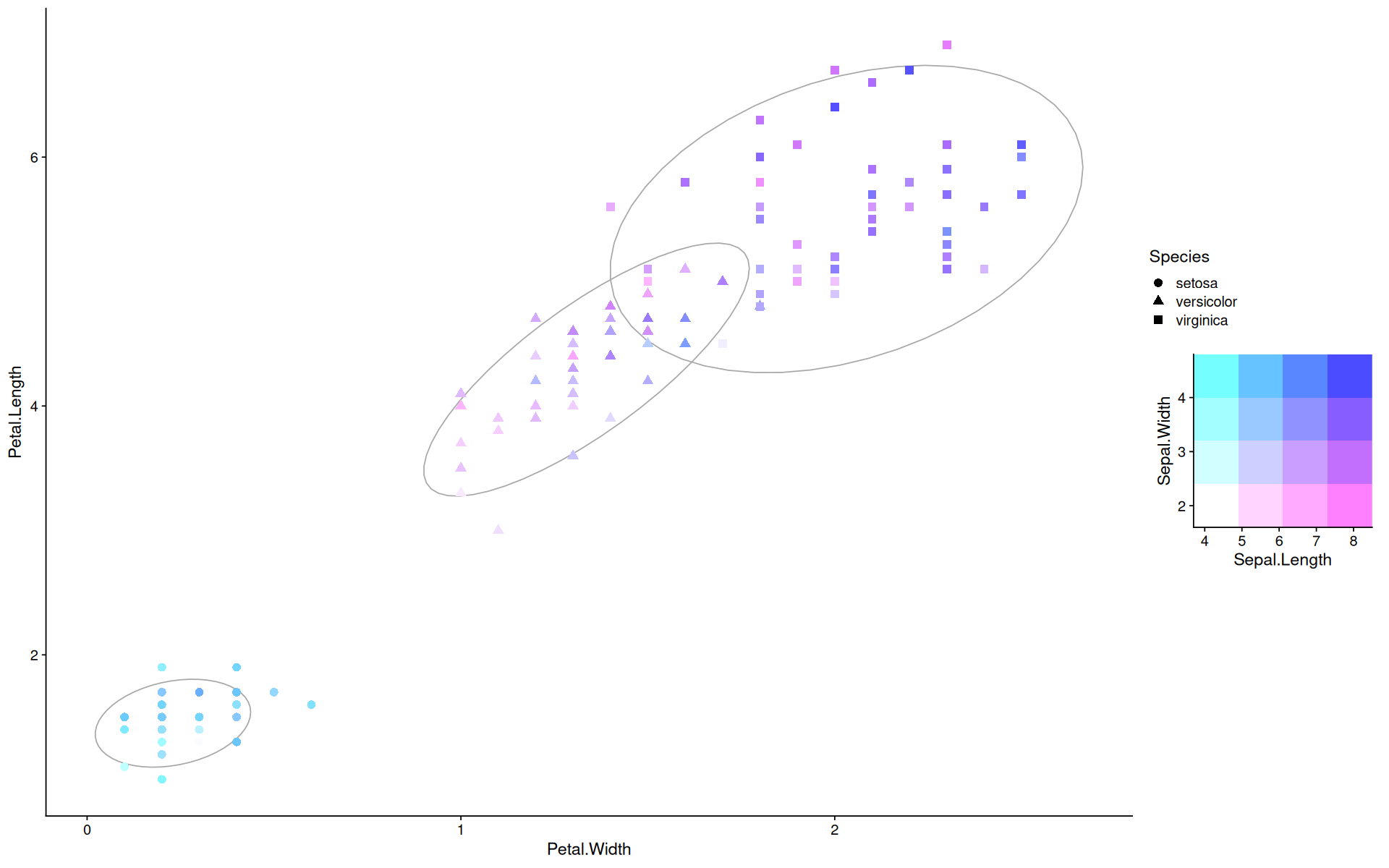
color(tolochko.redblue())<colors>
#DDDDDDFF #7BB3D1FF #016EAEFF #DD7C8AFF #8D6C8FFF #4A4779FF #CC0024FF #8A274AFF #4B264DFF color(tolochko.redblue()[c(9,3,1,7)])<colors>
#4B264DFF #016EAEFF #DDDDDDFF #CC0024FF r <- map_to_color2d(iris, xvar=Sepal.Length, yvar=Sepal.Width, colors=tolochko.redblue()[c(9,3,1,7)], size=3)
ggplot(r$data, aes(y=Petal.Length, x=Petal.Width, color=color, shape=Species, group=Species)) +
stat_ellipse(color='darkgray') +
geom_point(size=3) +
scale_color_identity() +
guides(custom = guide_custom(as_grob(r$legend), width=unit(0.4,'npc'), height=unit(0.4,'npc')))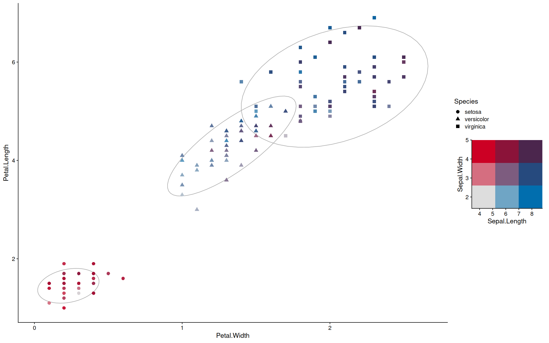
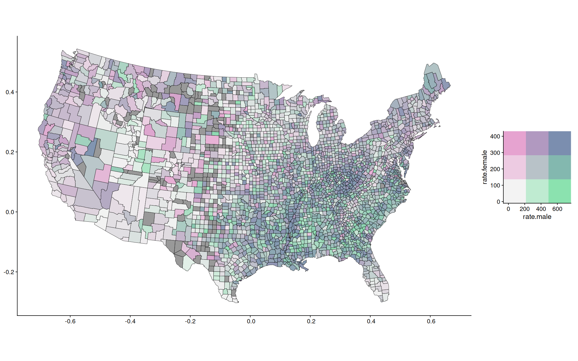
Choropleth
see also: https://
library(sf)Linking to GEOS 3.12.2, GDAL 3.9.0, PROJ 9.4.1; sf_use_s2() is TRUE
data(USCancerRates, package='latticeExtra')
data <-
    maps::map("county", fill=TRUE, plot =FALSE, projection = "tetra") |>
    st_as_sf() |>
    as_tibble() |>
    left_join(rownames_to_column(USCancerRates, 'ID'), by='ID')

head(data, 3)
Loading...
library(paletteer)data |>
ggplot(aes(fill=log2(rate.male/rate.female), geometry=geom)) +
geom_sf() +
scale_fill_paletteer_c(palette = 'grDevices::RdBu',limits=c(-1,1), oob=scales::squish, direction = -1)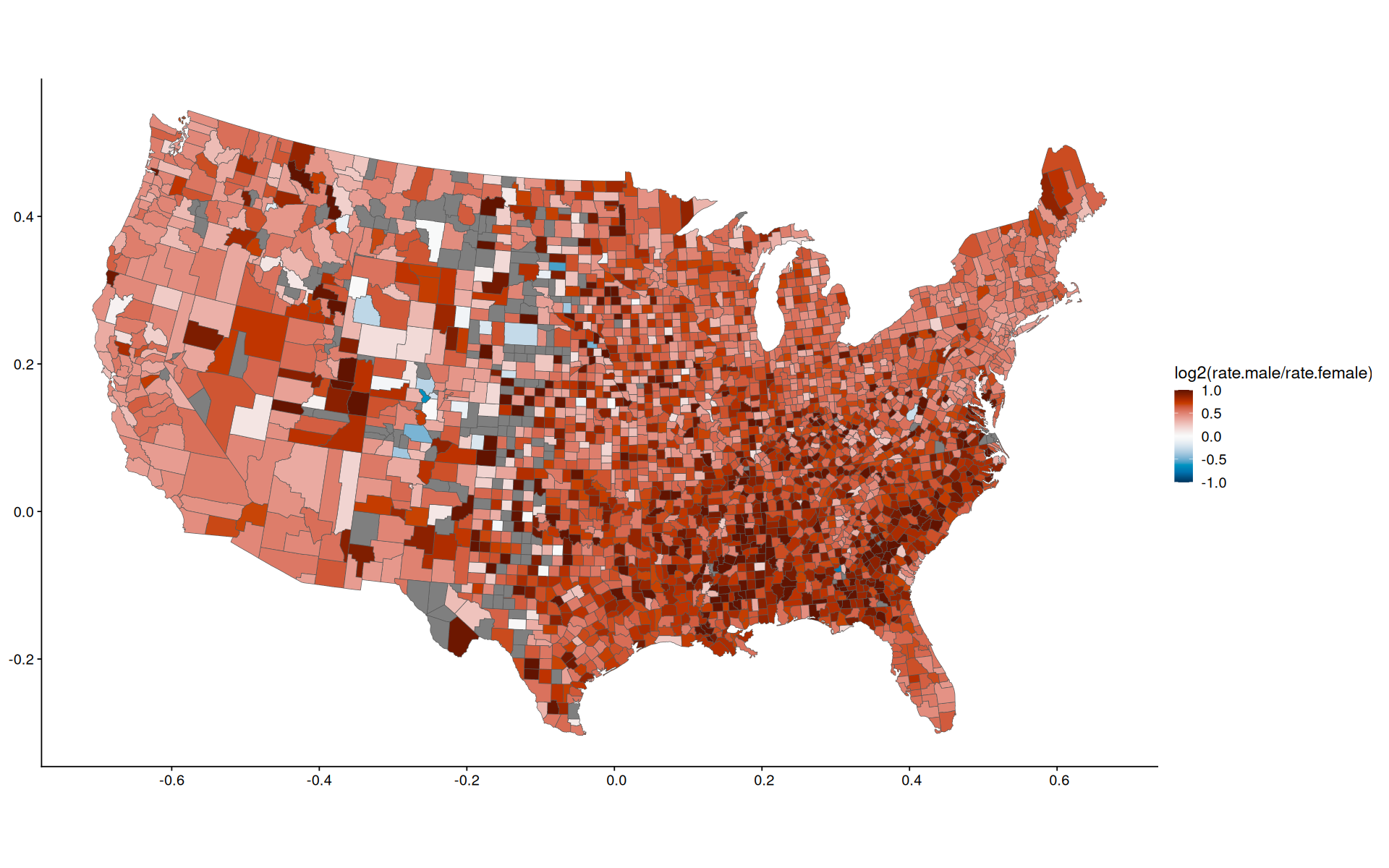
color(stevens.pinkgreen())<colors>
#F3F3F3FF #C2F1CEFF #8BE2AFFF #EAC5DDFF #9EC6D3FF #7FC6B1FF #E6A3D0FF #BC9FCEFF #7B8EAFFF color(stevens.pinkgreen()[c(9,3,1,7)])<colors>
#7B8EAFFF #8BE2AFFF #F3F3F3FF #E6A3D0FF r <- map_to_color2d(data, xvar=rate.male, yvar=rate.female, colors=stevens.pinkgreen()[c(9,3,1,7)], size=3, na.color='gray60')r$data |>
mutate(lab=ifelse(rate.female>400, ID, NA)) |>
ggplot(aes(fill=color, geometry=geom)) +
geom_sf(color='black') +
scale_fill_identity() +
guides(custom = guide_custom(as_grob(r$legend), width=unit(0.4,'npc'), height=unit(0.4,'npc')))